B02 — Roofline Model & Arithmetic Intensity¶
Track B · Module 02 · Status: DONE · Est. 6 hours · Depth 3/5
Prerequisites: A01 (kernels, error checking, event timing) and A02 (the measured bandwidth ladder this module turns into a model). Backends: AMD (
hipcc) · NVIDIA (nvcc) · Python (stdlib only, for the plotter). Setup: SETUP.md · Terms: GLOSSARY.md · Sources: REFERENCES.md.
1. TL;DR + Layman analogy¶
TL;DR. A kernel cannot go faster than two hard limits allow: the rate the machine can do
arithmetic (peak FLOP/s, call it P) and the rate it can move bytes
(bandwidth, B).
If a kernel does I FLOPs for every byte it pulls from memory, then bandwidth alone caps it at
I × B FLOP/s. Put the two together and you have the entire
roofline model:
I is the kernel's arithmetic intensity. The
intensity where the two limits meet is the
ridge point, I_ridge = P / B. Below it you are
memory-bound and the only lever that
matters is moving fewer bytes; above it you are compute-bound and the only lever that matters
is issuing better arithmetic. One division, one comparison, and you know which half of the
optimization literature to ignore.
Layman analogy — the restaurant kitchen. A chef can chop 100 ingredients a minute. The delivery van brings 10 ingredients a minute. However brilliant the chef, the kitchen produces 10 dishes' worth of prep a minute — the chef spends 90% of every minute waiting at the door. That kitchen is delivery-bound, and hiring a faster chef changes nothing; you need more vans, or you need recipes that do more work per ingredient (a stew that simmers for an hour off one crate beats a salad that consumes a crate a minute). Now flip it: give the kitchen twenty vans and the ingredients pile up in the corner, because the chef is the limit. Extra vans stop helping the moment deliveries outpace chopping. The ratio of chopping-per-ingredient is the arithmetic intensity, and the crossover where extra vans stop helping is the ridge point.
Where the analogy breaks — and it does, in three places you must know:
- It assumes a steady stream of orders. For a single sandwich, the dominant cost is the waiter walking to the kitchen and back. GPU equivalent: a kernel so small that launch overhead (~4 µs) dwarfs both ceilings. The roofline is silent about that entire regime.
- It assumes one chef with one skill. A real GPU has several compute ceilings — fp32
vector units, fp32 matrix cores, bf16 matrix cores, fp8 matrix cores, a slow transcendental
unit — each with its own
P, differing by more than 30×. Comparing against the wrong one gives a confidently wrong verdict. - It assumes the pantry does not exist. Real kitchens keep some ingredients on the shelf. A cache-resident working set changes the byte count entirely, which is why serious analysis uses a hierarchical roofline with one ceiling per memory level.
Section 6 makes all three concrete. A model whose failure modes you cannot state is a model you cannot trust.
%%{init: {
  'theme': 'base',
  'themeVariables': {
    'primaryColor': '#F8FAFC',
    'primaryTextColor': '#0F172A',
    'primaryBorderColor': '#0891B2',
    'lineColor': '#64748B',
    'secondaryColor': '#E0F2FE',
    'tertiaryColor': '#EEF2FF',
    'fontFamily': 'Inter, Segoe UI, sans-serif'
  }
}}%%
flowchart LR
  WORK["Work to do<br/>F FLOPs, M bytes"]
  T1["Arithmetic takes at least<br/>F / P seconds"]
  T2["Data movement takes at least<br/>M / B seconds"]
  MAX["With perfect overlap:<br/>time = max of the two"]
  RATE["attainable rate = F / time<br/>= min of P and I x B"]

  WORK --> T1 --> MAX
  WORK --> T2 --> MAX
  MAX --> RATE

  classDef trackB fill:#6366F1,stroke:#0F172A,color:#fff
  classDef neutral fill:#F8FAFC,stroke:#0891B2,color:#0F172A
  classDef success fill:#10B981,stroke:#0F172A,color:#fff
  class WORK neutral
  class T1,T2,MAX trackB
  class RATE success
Both branches are hard lower bounds on time; the model optimistically assumes they overlap perfectly, so it takes the larger of the two rather than their sum — remember that, because it is the first assumption to fail in practice.
By the end of this module you can: derive min(P, I × B) from scratch; compute the
arithmetic intensity of any operator in under a minute; find your machine's real ridge point by
measuring rather than reading a datasheet; place a measured kernel on the chart and name the
right next optimization; and state precisely where the model misleads you.
2. First Principles¶
Derive the whole model in four lines¶
Forget plots. Take a kernel that performs F floating-point operations and moves M bytes
between the GPU and HBM. The machine can retire at most P FLOP/s and move at most B bytes/s.
Two independent lower bounds on the runtime follow immediately:
time  >=  F / P          (you cannot do the arithmetic faster than the ALUs retire it)
time  >=  M / B          (you cannot get the data faster than the memory system delivers it)
If the two activities overlap perfectly — arithmetic on the data already resident while the next bytes are in flight — then the binding constraint is whichever is larger:
Now convert to a rate, because that is what people quote. Divide F by the time and define
the arithmetic intensity I = F / M:
rate  =  F / time  <=  F / max(F/P, M/B)
                    =  min(F / (F/P),  F / (M/B))
                    =  min(P,  (F/M) x B)
                    =  min(P,  I x B)
That is the roofline, in the form Williams, Waterman and Patterson published it in 2009, and the ridge-point vocabulary below is theirs too. Everything else in this module — every operator table, every diagram, every profiler chart — is bookkeeping on those two terms.
The load-bearing assumption is
max, not+. If a kernel cannot overlap loads with math at all, the honest bound istime >= F/P + M/B, which is up to 2× worse. The roofline takes the optimistic branch on the grounds that GPUs are built to overlap (many resident warps, one stalls while another computes). When a kernel has too few warps to overlap, the model becomes an optimistic fiction — see Section 6.
Arithmetic intensity, defined precisely¶
The second half of that sentence carries all the subtlety. "Bytes moved" is not the size of the tensors, and not the bytes your code asked for. It is the traffic that actually crossed the boundary you care about:
| If you model... | Then bytes means... | And the ceiling B is... |
|---|---|---|
| HBM / device memory | traffic between L2 and HBM | achievable HBM bandwidth |
| L2 | traffic between L1 and L2 | achievable L2 bandwidth |
| L1 / LDS | traffic between registers and L1 | achievable L1 bandwidth |
Three consequences that trip people up:
- A cache-resident working set changes the answer. A 16 KB row read five times generates
5 × 16 KBof L1/L2 traffic but only16 KBof HBM traffic. Its HBM intensity is 5× its L2 intensity. Both numbers are correct; they answer different questions. This is exactly why hierarchical rooflines exist (Yang, Kurth & Williams — see Section 8). - Wasted bytes count. An uncoalesced kernel that fetches 128-byte lines to use 4 bytes of each moves 32× the bytes it needed. Its measured intensity collapses by 32×, and it will sit neatly on a roofline it should never have been anywhere near. Always compare against the intensity of the ideal implementation, not the one you wrote.
Iis a property of the algorithm and its data layout, not of the GPU. Vector add hasI = 1/12on every device ever built. What changes between devices is the ridge point you compare it against.
The ridge point, and why it is absurdly high now¶
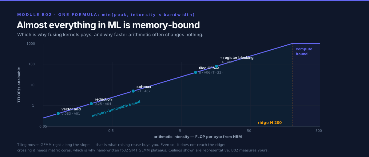
Every kernel this curriculum builds sits on the slanted part. The flat compute-bound region to the right of the ridge is almost empty — that emptiness is why fusion pays and why faster arithmetic so often changes nothing.
Set the two terms of min(P, I × B) equal:
This single number tells you the intensity a kernel must exceed to be limited by arithmetic rather than by memory. Here it is for two current data-center parts, from vendor-published peak specifications (these are datasheet numbers, not measurements — Lab 1 measures the real ones):
| Device | B (HBM) |
Compute ceiling | P |
I_ridge = P/B |
|---|---|---|---|---|
| AMD MI300X | 5.3 TB/s | fp32 vector | 81.7 TFLOP/s | 15.4 FLOP/byte |
| AMD MI300X | 5.3 TB/s | fp32 matrix | 163.4 TFLOP/s | 30.8 |
| AMD MI300X | 5.3 TB/s | fp16/bf16 matrix | 1307.4 TFLOP/s | 246.7 |
| AMD MI300X | 5.3 TB/s | fp8 matrix | 2614.9 TFLOP/s | 493.4 |
| NVIDIA H100 SXM | 3.35 TB/s | fp32 vector | 66.9 TFLOP/s | 20.0 |
| NVIDIA H100 SXM | 3.35 TB/s | TF32 tensor | 494.7 TFLOP/s | 147.7 |
| NVIDIA H100 SXM | 3.35 TB/s | bf16 tensor | 989.4 TFLOP/s | 295.3 |
| NVIDIA H100 SXM | 3.35 TB/s | fp8 tensor | 1978.9 TFLOP/s | 590.7 |
Read the bolded rows and then read this: a bf16 matrix-core kernel must do about 250–300 floating-point operations for every single byte it reads from HBM before arithmetic becomes its limit. A vector add does 0.083. That is a factor of roughly 3,000.
This is the most important number in ML performance engineering, and it explains the shape of the entire field:
- Matrix cores made
Pgrow by more than 20× in a few generations.Bgrew by perhaps 3×. So the ridge point marched right, and kernels that used to be near it are now far to its left. - Faster compute makes more kernels memory-bound, not fewer. Every elementwise op, every normalization, every attention softmax, the entire decode phase of inference — all of them are pinned to the bandwidth roof on modern hardware.
- Which is why the dominant optimizations of the last five years are all byte-deleting techniques: kernel fusion, FlashAttention, quantization, activation checkpointing trade-offs, paged KV caches. None of them make the math faster. They make there be less traffic.
%%{init: {
  'theme': 'base',
  'themeVariables': {
    'primaryColor': '#F8FAFC',
    'primaryTextColor': '#0F172A',
    'primaryBorderColor': '#0891B2',
    'lineColor': '#64748B',
    'secondaryColor': '#E0F2FE',
    'tertiaryColor': '#EEF2FF',
    'fontFamily': 'Inter, Segoe UI, sans-serif'
  }
}}%%
flowchart LR
  ZERO["low intensity<br/>attainable rate near zero"]
  SLOPE["RISING ROOF<br/>attainable = I x B<br/>slope is memory bandwidth<br/>MEMORY-BOUND"]
  RIDGE["RIDGE POINT<br/>I_ridge = P / B<br/>both roofs bind here"]
  FLAT["FLAT ROOF<br/>attainable = P<br/>slope is zero<br/>COMPUTE-BOUND"]
  ZERO --> SLOPE --> RIDGE --> FLAT

  VADD["vector add fp32<br/>I = 0.083"]
  RED["sum reduction fp32<br/>I = 0.25"]
  SOFT["fused softmax fp32<br/>I = 0.625"]
  ATTN["unfused attention bf16<br/>I approx 64 at ANY s"]
  GEMM["GEMM fp32 N=8192<br/>I = 1365"]
  FLASH["fused attention bf16 s=8192<br/>I = 4136"]

  VADD -.-> SLOPE
  RED -.-> SLOPE
  SOFT -.-> SLOPE
  ATTN -.-> SLOPE
  GEMM -.-> FLAT
  FLASH -.-> FLAT

  classDef trackB fill:#6366F1,stroke:#0F172A,color:#fff
  classDef warn fill:#FEF3C7,stroke:#F59E0B,color:#0F172A
  classDef success fill:#10B981,stroke:#0F172A,color:#fff
  classDef neutral fill:#F8FAFC,stroke:#0891B2,color:#0F172A
  class SLOPE,FLAT,RIDGE trackB
  class VADD,RED,SOFT,ATTN warn
  class GEMM,FLASH success
  class ZERO neutral
Mermaid cannot draw a log-log plot, so this is the roofline's shape rendered as a diagram:
a line rising with slope B, a knee at the ridge point, then a horizontal ceiling at P, with
real operators hung underneath the region they land in — and note that four of the six sit on
the rising part, which is the whole story of ML kernels. For an actual plotted chart with axes,
run tools/roofline_plot.py (Lab 3).
3. Deep Dive¶
Worked arithmetic intensity for real operators¶
The skill is mechanical once you have seen it done. For each operator: count FLOPs, count the
bytes that must cross HBM in the best possible implementation, divide. Conventions used
throughout: one FMA is 2 FLOPs, exp is charged as 1 FLOP, fp32 is 4 bytes.
Elementwise — C[i] = A[i] + B[i]¶
per element:  1 add                      ->  1 FLOP
              read A (4) + read B (4) + write C (4)  ->  12 bytes
I = 1 / 12 = 0.083 FLOP/byte
Against MI300X's bf16 ridge of 247, this is 2,960× too low. There is no tuning, no block size, no occupancy trick that makes vector add compute-bound. Its only possible optimization is to stop being a separate kernel — which is what fusion means. This formalizes what A01 §5 sketched.
Reduction — sum(A)¶
per element:  1 add                      ->  1 FLOP
              read A (4)                 ->  4 bytes   (the output is one scalar; ignore it)
I = 1 / 4 = 0.25 FLOP/byte
Three times better than vector add purely because there is nothing to write back. Still 1,000× below the ridge. A good reduction is judged by what fraction of the copy ceiling it reaches, never by its GFLOP/s — a point A04 §5 makes with code and this module makes with a model.
Softmax — and why fusion is the whole game¶
The textbook safe softmax is three passes over the row (find the max, exponentiate, normalize):
FLOPs per element:  max compare (1) + subtract (1) + exp (1) + accumulate (1) + divide (1) = 5
bytes, 3-pass:      pass 1 reads 4; pass 2 reads 4 writes 4; pass 3 reads 4 writes 4  = 20
I_3pass = 5 / 20 = 0.25 FLOP/byte

bytes, fused single pass (online normalization): read 4, write 4  = 8
I_fused = 5 / 8 = 0.625 FLOP/byte
2.5× the intensity, identical arithmetic, identical output. The single-pass form is the online normalizer of Milakov and Gimelshein (2018), which is what makes one pass numerically safe. Both are still deeply memory-bound — the classification did not change — but the fused version's roof is 2.5× higher, so it finishes 2.5× sooner. Internalize this: fusion rarely changes your verdict; it moves you up the memory-bound slope by deleting bytes. That is the model's prediction for A07 §5, which measures it.
GEMM — the operator that escapes¶
Square N × N × N matrix multiply, element size s bytes. Perfect tiling means each of A, B, C
crosses HBM exactly once, i.e. 3N² elements:
Intensity grows linearly with N. That is what makes GEMM
the only major ML primitive that
is genuinely compute-bound — and only once it is big enough. Solving 2N/(3s) >= I_ridge:
| Precision | s |
I(N) |
MI300X ridge | Smallest compute-bound N |
|---|---|---|---|---|
| fp32 (vector) | 4 | N/6 |
15.4 | 93 |
| fp32 (matrix) | 4 | N/6 |
30.8 | 185 |
| bf16 (matrix) | 2 | N/3 |
246.7 | 741 |
| fp8 (matrix) | 1 | 2N/3 |
493.4 | 741 |
Two things to notice. First, a bf16 GEMM smaller than about N = 740 is memory-bound on
MI300X — which is why small-batch inference GEMMs and thin projection layers behave nothing
like the GEMM in the benchmarks. Second, fp8 and bf16 need the same N: dropping to fp8
doubles P and halves the bytes, and the two effects cancel exactly for GEMM. For
memory-bound operators there is no such cancellation, and halving the bytes is a clean 2× win.
That asymmetry is the real reason quantization pays off more on the memory-bound parts of a model
than on its GEMMs.
Also notice what the 3N² assumed: perfect reuse. A naive one-thread-per-output kernel reads
a full row and column per output element, moving 2N³ elements instead of 3N² — intensity
collapses to 2N³/(2N³ × 4) = 0.25 FLOP/byte, the same as a reduction, no matter how large N
gets. Tiling is not a 20% optimization; it is the difference
between I = 0.25 and I = N/6.
A06 §4 builds
exactly that.
Attention — memory-bound unless fused¶
One head, sequence length s, head dimension d, bf16. FLOPs are dominated by the two GEMMs:
F = 4s²d + 5s². The byte count depends entirely on whether the s × s score matrix touches
HBM:
unfused (QK^T, softmax, PV as three kernels):
    bytes = 8sd + 8s²          (score matrix written once, read twice)
    I     = s(4d + 5) / (8(d + s))     ->  (4d + 5)/8  ~=  d/2   as s grows

fused (FlashAttention-style, score matrix stays on chip):
    bytes = 8sd                (Q, K, V read once; O written once)
    I     = s(4d + 5) / (8d)           ->  grows linearly in s
At d = 128 the unfused intensity converges to 64.6 FLOP/byte and stays there — 512, 8192,
or 32768 tokens, it barely moves, because its traffic is O(s²) and grows exactly as fast as its
FLOPs. Against MI300X's bf16 ridge of 247 it is memory-bound at every sequence length; the
inequality has no solution. The fused version is ≈ 0.505 s, crossing the ridge at
s ≈ 490 on MI300X and staying compute-bound forever after.
That is FlashAttention's justification stated as an inequality rather than an anecdote — the
IO-complexity argument of
Dao et al. (2022) in two lines of
byte counting — and it is why
A09 §2
treats fused attention as an algorithm change rather than an optimization. Exercise 2 walks the
full derivation, including the causal, decode, and
grouped-query variants — decode attention lands at I ≈ 1 FLOP/byte, which is why token
generation throughput tracks HBM bandwidth almost linearly.
%%{init: {
  'theme': 'base',
  'themeVariables': {
    'primaryColor': '#F8FAFC',
    'primaryTextColor': '#0F172A',
    'primaryBorderColor': '#0891B2',
    'lineColor': '#64748B',
    'secondaryColor': '#E0F2FE',
    'tertiaryColor': '#EEF2FF',
    'fontFamily': 'Inter, Segoe UI, sans-serif'
  }
}}%%
flowchart TB
  Q["What sets this operator's intensity?"]
  Q --> E["Elementwise / normalization<br/>I fixed by dtype and op count<br/>0.08 to 0.6 FLOP/byte"]
  Q --> R["Reduction<br/>I fixed, no output traffic<br/>0.25 FLOP/byte"]
  Q --> G["GEMM<br/>I grows with tile size and N<br/>2N / 3s FLOP/byte"]
  Q --> A["Attention<br/>I depends on FUSION, not on s<br/>d/2 unfused vs 0.5s fused"]

  E --> EF["Only lever: delete bytes<br/>fuse, in-place, smaller dtype"]
  R --> RF["Already optimal<br/>score as percent of copy ceiling"]
  G --> GF["Tile for reuse, then chase<br/>matrix-core utilization"]
  A --> AF["Fuse first, everything else second"]

  classDef trackB fill:#6366F1,stroke:#0F172A,color:#fff
  classDef warn fill:#FEF3C7,stroke:#F59E0B,color:#0F172A
  classDef success fill:#10B981,stroke:#0F172A,color:#fff
  classDef neutral fill:#F8FAFC,stroke:#0891B2,color:#0F172A
  class Q neutral
  class E,R,A warn
  class G trackB
  class EF,RF,GF,AF success
Four operator families, four different reasons their intensity is what it is — and the point of the diagram is that the lever falls out of the intensity's structure, not out of guesswork.
AMD vs NVIDIA: same model, different ceilings and different names¶
| Concept | AMD CDNA3 (MI300X) | NVIDIA Hopper (H100) |
|---|---|---|
| Vector FLOP unit | VALU (v_fma_f32), 64-lane wavefront |
CUDA cores (FFMA), 32-lane warp |
| Matrix unit | Matrix Core, MFMA instructions |
Tensor Core, HMMA/QGMMA instructions |
| HBM ceiling | HBM3, 5.3 TB/s | HBM3, 3.35 TB/s |
| On-chip level worth modelling | LDS (64 KB/CU), L2, Infinity Cache | Shared memory (up to 228 KB/SM), L2 (50 MB) |
| Built-in roofline tool | rocprof-compute (ROCm Compute Profiler), --roof-only |
Nsight Compute, --set roofline or --set full |
| HBM byte counters | FETCH_SIZE, WRITE_SIZE |
dram__bytes_read.sum, dram__bytes_write.sum |
| fp32 FLOP counters | VALU FLOP counters (rocprof-compute derives them) |
sm__sass_thread_inst_executed_op_ffma_pred_on.sum (×2), plus fadd/fmul |
Note that both vendors ship an empirical roofline: neither tool reads peaks off a datasheet.
rocprof-compute runs its own microbenchmarks to establish the ceilings and stores them in
roofline.csv; Nsight Compute derives them from measured achievable throughputs. Lab 1 is a
hand-rolled version of the same idea, and doing it yourself once is what makes the tools' output
legible.
How to place a real kernel on the roofline¶
Five steps, in this order. Do not skip step 5.
- Count FLOPs analytically. From the algorithm, not from a counter.
2N³for a GEMM,4s²dfor attention. Analytic counts are what you should be doing; hardware counters tell you what you did, including waste. You want both, and the gap between them is informative. - Get bytes. Analytically for the ideal implementation, and from the profiler for the real
one (
FETCH_SIZE/WRITE_SIZE, ordram__bytes_*). A large ratio between the two is an access-pattern bug, not a roofline result — go back to A02 §3. - Compute
Iand the roof.I = FLOPs / bytes;roof = min(P, I × B)withPandBfrom Lab 1, not from a datasheet. - Compute achieved FLOP/s from your measured kernel time, and plot the point.
- Compare achieved to roof, then act. The decision rule:
| Situation | What it means | What to do next |
|---|---|---|
I < I_ridge and achieved ≈ roof |
Memory-bound and bandwidth-optimal | Reduce bytes: fuse, raise reuse via tiling/shared memory, use a smaller dtype, avoid materializing intermediates. Nothing else will help. |
I > I_ridge and achieved ≈ roof |
Compute-bound and near peak | Improve the instruction mix: use matrix cores, packed ops, fewer transcendentals; then raise ILP or occupancy. |
| achieved « roof (say < 50%) | Bound by something the roofline does not model | Do not optimize bytes or FLOPs yet. Check occupancy, warp-stall reasons, launch size, register spills, and tail effects. Section 6. |
I near I_ridge |
Both roofs bind | Check load/math overlap (software pipelining, prefetch), then re-measure. |
Step 5's third row is the one that separates engineers who have used a roofline from engineers who have read about one.
4. Hands-On Labs¶
All commands run from this module directory. There is no triton/ directory here: the module's
subject is a model, and the labs that matter are microbenchmarks that must control instruction
selection and memory traffic precisely — which is exactly what a high-level DSL abstracts away.
Triton kernels are analyzed with this model in
A08 and
B03.
# AMD
make hip GPU_ARCH=gfx942     # build hip/ programs
make run-hip                 # ceilings first, then the intensity sweep

# NVIDIA
make cuda SM_ARCH=sm_90      # build cuda/ programs
make run-cuda

# Roofline chart (any machine, no GPU needed, stdlib Python only)
make plot
The drills are self-contained too: exercises/ and solutions/
each have their own Makefile, so you can cd exercises && make run without coming back here.
From this directory, make exercises / make solutions build them in place, and make clean
cleans all three.
Match
GPU_ARCHto your GPU.gfx950= MI350,gfx942= MI300,gfx90a= MI200,gfx1100= RDNA3. Find yours with/opt/rocm/bin/offload-arch(orrocminfo | grep gfx). Troubleshooting forlibamdhip64.soandhipErrorNoBinaryForGpuis in A01 §4; this module shares Track A'scommon.mk, so the same rpath fix applies.
Lab 1 — Measure your two ceilings (measure_ceilings)¶
Files: hip/measure_ceilings.cpp ·
cuda/measure_ceilings.cu.
Two microbenchmarks, one per axis:
copy_kernel— a fully coalesced grid-stride copy, the most bandwidth-friendly kernel that can exist. Its GB/s is your memory roofB. (This is A02'sbandwidthlab, reused deliberately: the ladder you measured there is the axis you are now drawing.)fma_peak_kernel— a register-resident FMA loop with 8 independent chains and one store per thread for the whole kernel. Its GFLOP/s is your compute roofP.
What to observe: the printed ridge point I_ridge = P / B. Write it down; every verdict in
this module is relative to it. Then compare B to your GPU's datasheet HBM peak — you should
land at a healthy fraction, and the achievable number is the honest one to build a model on.
Two design details worth understanding, because they are the difference between a measurement and a mistake:
- Why 8 independent chains? One dependent chain (
v = fma(v, a, b)over and over) measures FMA latency, not throughput: each instruction waits for the previous one. With enough independent chains per thread the scheduler always has a ready instruction, and you measure the pipeline's issue rate. A single-chain version of this kernel can under-report peak by several times, which would put a false floor under your entire roofline. - Why
a = 1.0f, b = 0.0f? The chain becomes the identity, so the expected output is exactly the sum of the seeds and verification is bit-exact. The compiler cannot fold the FMAs away becauseaandbare runtime kernel arguments it cannot see, and IEEE-754 semantics forbid reassociating them. You get a benchmark that is simultaneously trivially verifiable and honestly doing the work.
Lab 2 — Discover the ridge point empirically (roofline_sweep)¶
Files: hip/roofline_sweep.cpp ·
cuda/roofline_sweep.cu.
This is the key lab, and its design is the lesson. One kernel with arithmetic intensity as a
tunable parameter. Every thread loads a float, applies K fused multiply-adds to it in
registers, and stores it. Bytes per element are fixed at 8; FLOPs per element are 2K. So:
Sweeping K ∈ {0, 1, 2, 4, ..., 512} walks I from 0 to 128 FLOP/byte — a single kernel
traversing the entire roofline. K is a template parameter, not a kernel argument, so the
FMA sequence unrolls into straight-line code and no loop overhead pollutes the low-K end where
the measurement is most delicate. Four independent chains per thread keep the high-K end
throughput-bound rather than latency-bound, for the same reason as Lab 1.
What to observe. Two tables. The first is raw: per K, the achieved GB/s and GFLOP/s. The
second places each point against the ceilings and prints a bar. The shape to look for:
- At small
K: GB/s pins near the copy ceiling; GFLOP/s is tiny. The kernel is doing almost nothing but moving data — you are on the rising roof. - As
Kgrows: GFLOP/s climbs roughly linearly (doubleK, double the rate) while GB/s holds. The extra arithmetic is free, hidden behind memory traffic that was happening anyway. This is the single most counter-intuitive fact in GPU performance, and here you watch it happen. - At large
K: GFLOP/s flattens against the compute roof and GB/s collapses. Adding arithmetic now costs time linearly. - The knee between the two regimes is the ridge point — and the program computes it from the
two extremes of its own sweep (
I_ridge = max GFLOP/s ÷ max GB/s) rather than asserting it.
K = 0 is the pure-copy case, which is how the sweep calibrates its own bandwidth roof without
needing Lab 1's numbers passed in.
Every row verifies. Because a = 1.0f and b = 0.0f, the output must equal the input
bit-for-bit for every K. A sweep whose fast points are fast because they are wrong is worse
than no sweep.
Expect hardware-specific numbers and a hardware-independent shape. Where your knee lands depends on your GPU, its clocks, and its thermal state. That there is a knee, that GFLOP/s rises then flattens, and that GB/s does the mirror image — that is universal. Do not compare your absolute numbers to anyone else's; compare your ridge point to your operators' intensities.
This is the slowest file in the curriculum to compile (tens of seconds). The
K = 256andK = 512instantiations unroll into a couple of thousand FMA instructions each, which is the price of measuring throughput rather than loop overhead.
Lab 3 — Draw the chart and classify (tools/roofline_plot.py)¶
File: tools/roofline_plot.py. Pure standard library — no numpy, no
matplotlib — so it runs on a bare login node.
# with the ceilings Lab 1 printed for your machine
python tools/roofline_plot.py --peak-gflops 78500 --peak-gbps 4650 --demo-kernels

# add your own kernel; numeric fields accept the formula, not just the product
python tools/roofline_plot.py --peak-gflops 78500 --peak-gbps 4650 \
    --kernel "my_softmax, 5*2**24, 8*2**24, 410"

# illustrative ceilings, for when you have no GPU in front of you
make plot
It prints an ASCII log-log roofline (# for the roof, : for the ridge, letters for kernels)
plus a table giving each kernel's intensity, its roof, the fraction of that roof it reached, and
the next step you should take. The --kernel spec is name, flops, bytes[, achieved_gflops];
pass the achieved rate and the tool will tell you when a kernel is far below its own roof and
therefore not bound by the roof you were about to optimize against.
What to observe: how brutally left-of-ridge the entire elementwise/reduction/softmax family is, and how far the fused GEMM and attention points are from them. The chart makes the 3,000× gap from Section 2 visceral in a way the table does not.
Lab 4 (optional) — Compare against the vendors' own rooflines¶
# AMD: runs its own ceiling microbenchmarks, then plots your kernels
rocprof-compute profile -n b02_sweep --roof-only -- ./hip/roofline_sweep.exe
rocprof-compute analyze -p workloads/b02_sweep/MI300X

# NVIDIA
ncu --set roofline -o b02_sweep ./cuda/roofline_sweep.exe     # then open in the Nsight Compute UI
make profile-hip        # or: make profile-cuda   (timeline-level view)
What to look for: the vendor tools' ceilings should be close to Lab 1's — if rocprof-compute
or Nsight Compute reports a compute roof much higher than yours, your FMA loop is not saturating
the pipes (chains, occupancy, or instruction selection). More importantly, look at the
hierarchical roofline both tools offer: the same kernel plotted against L1, L2, and HBM
ceilings simultaneously. A kernel that looks memory-bound against HBM but sits at the L2 ceiling
has a cache problem, not a bandwidth problem — a distinction the single-level model in
Section 2 physically cannot express.
5. Performance Analysis¶
The recipe, applied¶
The point of this module is that "is it memory- or compute-bound?" becomes a two-minute arithmetic exercise rather than an opinion. Concretely, for any kernel:
I        = FLOPs / bytes                     <- analytic, plus profiler bytes for the real thing
roof     = min(P, I x B)                     <- P and B from measure_ceilings, not a datasheet
achieved = FLOPs / measured_seconds
verdict  = compare I to I_ridge, then compare achieved to roof
Expected shape of the sweep¶
roofline_sweep computes every number below at run time, so this table gives the shape, with
<measured> where your hardware decides. The intensity column is analytic and must match
exactly — it is K/4 by construction.
K |
I (FLOP/byte) |
GB/s | GFLOP/s | regime |
|---|---|---|---|---|
| 0 | 0.00 | <measured> — this is your B |
0 | bandwidth calibration |
| 1 | 0.25 | ≈ B |
small, ≈ 0.25 B |
memory-bound |
| 4 | 1.00 | ≈ B |
≈ 1.0 B |
memory-bound |
| 16 | 4.00 | ≈ B |
≈ 4.0 B |
memory-bound |
| 64 | 16.00 | falling | rising | approaching the ridge |
| 128 | 32.00 | well below B |
≈ P |
compute-bound |
| 512 | 128.00 | far below B |
<measured> — this is your P |
compute-bound |
The signature to look for: a rising line that flattens. GFLOP/s roughly doubles with each
doubling of K while the kernel is on the memory roof, then stops responding once it hits the
compute roof. B and P are read off the two ends of the sweep, and their ratio is the ridge
point. Nothing here is asserted; the transition is located by the measurement.
On current data-center parts the knee should appear somewhere around I = 15–30 FLOP/byte
(K ≈ 60–120) for fp32, consistent with the datasheet ridge points in Section 2 — but treat that
as a prediction the lab either confirms or refutes on your hardware, not as an expected result.
Reading a memory-bound kernel correctly¶
For a kernel with I far left of the ridge, GFLOP/s is the wrong headline. Consider
A02 §5's
transpose ladder, measured there on an MI300X (gfx942, ROCm 6.2) — transpose does zero
arithmetic, so I = 0 and the roofline degenerates to the bandwidth axis alone:
| Kernel (from A02) | I |
Measured BW | % of A02's measured copy ceiling |
|---|---|---|---|
bandwidth (copy) |
0 | ~4800 GB/s | ceiling |
transpose_naive |
0 | ~700 GB/s | ~15% |
transpose_tiled |
0 | ~2600 GB/s | ~54% |
transpose_tiled_padded |
0 | ~3400 GB/s | ~70% |
Those are A02's numbers, not new measurements. What B02 adds is the interpretation: with
I = 0 there is no compute roof to reach and no FLOP/s worth quoting, so the only meaningful
score is percentage of achievable bandwidth. The naive kernel is not "slow at math"; it is
moving roughly 5× more bytes than the problem requires because its writes are uncoalesced. The
roofline's honest verdict on a zero-FLOP kernel is: go look at your access pattern.
A before/after the model predicts in advance¶
Softmax, from Section 3, is the cleanest case where the model makes a falsifiable prediction before any code is written:
| Version | FLOPs | HBM bytes | I |
Predicted speedup |
|---|---|---|---|---|
| 3-pass safe softmax | 5N |
20N |
0.25 | baseline |
| Fused single-pass | 5N |
8N |
0.625 | 2.5× |
Both are memory-bound, so runtime is bytes / B in each case and the ratio is exactly
20N / 8N = 2.5. If A07's
fused kernel measures ~2.5× and not ~5×, the model was right and the
implementation is fine. If it measures 1.2×, the model is telling you the fused version is not
actually achieving bandwidth — go find out why. A model earns its place by being wrong in
informative ways, and that only works if you commit to the prediction first.
6. Challenges, Drawbacks & Tradeoffs¶
The roofline is the most useful performance model in GPU engineering, and it is wrong in at least nine identifiable ways. Knowing them is the difference between a tool and a talisman.
%%{init: {
  'theme': 'base',
  'themeVariables': {
    'primaryColor': '#F8FAFC',
    'primaryTextColor': '#0F172A',
    'primaryBorderColor': '#0891B2',
    'lineColor': '#64748B',
    'secondaryColor': '#E0F2FE',
    'tertiaryColor': '#EEF2FF',
    'fontFamily': 'Inter, Segoe UI, sans-serif'
  }
}}%%
flowchart TD
  START{"Kernel far below<br/>its roofline?"}
  START -->|"kernel runs for only a few microseconds"| L1["Launch- or latency-bound<br/>roofline never applies"]
  START -->|"occupancy is low"| L2["Not enough warps to hide latency<br/>the max() overlap assumption failed"]
  START -->|"L2 hit rate is high"| L3["You modelled the wrong level<br/>need a hierarchical roofline"]
  START -->|"kernel uses fp16 or bf16 matrix ops"| L4["Wrong compute ceiling<br/>compared against fp32 peak"]
  START -->|"lots of exp, sqrt, div"| L5["Transcendental unit, not FMA<br/>your P does not apply"]
  START -->|"bytes moved much greater than bytes needed"| L6["Access-pattern bug<br/>fix coalescing before modelling"]

  L1 --> F1["Batch work, fuse, use graphs<br/>or keep it on the CPU"]
  L2 --> F2["Raise occupancy or ILP<br/>check registers and LDS per block"]
  L3 --> F3["Plot against L1, L2 and HBM<br/>ncu --set roofline / rocprof-compute"]
  L4 --> F4["Re-plot against the matrix-core peak"]
  L5 --> F5["Measure a transcendental ceiling too<br/>or cut the transcendental count"]
  L6 --> F6["Back to A02: coalesce, then re-measure"]

  classDef trackB fill:#6366F1,stroke:#0F172A,color:#fff
  classDef warn fill:#FEF3C7,stroke:#F59E0B,color:#0F172A
  classDef success fill:#10B981,stroke:#0F172A,color:#fff
  class START trackB
  class L1,L2,L3,L4,L5,L6 warn
  class F1,F2,F3,F4,F5,F6 success
Six of the nine failure modes as a triage tree — note that every branch ends in "the roofline is not your problem yet," which is the most common state a real kernel is in.
Pitfall 1 — The latency-bound regime is invisible¶
The roofline has no axis for latency. It silently assumes the kernel runs long enough to reach steady state with enough parallelism to saturate whichever unit binds. A kernel with 4 resident warps per SM, or one that runs for 3 µs, is limited by neither roof — it is limited by instruction and memory latency it has no other work to hide behind, and by the ~4 µs it costs to launch it at all.
Concretely: a 4096-element fp32 vector add moves 49 KB. At 4 TB/s that traffic takes 12 nanoseconds, against a launch overhead of roughly 4,000 ns — a factor of 325. Its intensity is identical to the 64-million-element version, so the roofline gives an identical, useless verdict. A point far below its own roof is the model telling you it does not apply. That is not a failure to read past; it is the single most valuable signal the chart produces.
Pitfall 2 — Perfect overlap is assumed, not achieved¶
Section 2 derived time >= max(F/P, M/B). The pessimistic bound is F/P + M/B. A kernel with a
strictly serial structure — load a tile, barrier, compute it, barrier, load the next — approaches
the sum and can therefore sit at 50% of its roofline while being perfectly well written for its
structure. Software pipelining, double buffering, and asynchronous copies
(cp.async / buffer_load_dword ... lds) exist to close exactly this gap. The roofline scores
the outcome; it never tells you overlap was the missing ingredient.
Pitfall 3 — There is no cache in the model¶
The single-level roofline pretends memory is one flat pool at bandwidth B. Real GPUs have
registers, LDS/shared memory, L1, L2, and (on MI300X) Infinity Cache — differing by orders of
magnitude in both bandwidth and latency. Two consequences:
- A kernel whose working set fits in L2 moves far fewer HBM bytes than a naive count suggests, so its true HBM intensity is much higher than you computed and it may not be HBM-bound at all.
- A kernel can be L2-bandwidth-bound while sitting comfortably below the HBM roof. On the single-level chart it looks like an unexplained underperformer.
The fix is the hierarchical roofline: one ceiling per level, the kernel plotted against all of them (Yang, Kurth & Williams; both vendors' profilers implement it). This is not an academic refinement — it is the difference between "add more reuse" and "your reuse is already working, the problem is L2 throughput."
Pitfall 4 — There is more than one compute ceiling¶
P is not a property of a GPU; it is a property of a GPU and an instruction mix. MI300X has
at least four meaningfully different compute roofs (fp32 vector 81.7, fp32 matrix 163.4, bf16
matrix 1307.4, fp8 matrix 2614.9 TFLOP/s) spanning 32×. Pick the wrong one and:
- Comparing a bf16 matrix-core kernel against the fp32 ceiling makes it look compute-bound when
it is memory-bound, and sends you off optimizing arithmetic that was never the problem.
(Exercise 1 row 8 is exactly this trap:
I = 124 FLOP/byteis compute-bound against a ridge of 15 and memory-bound against a ridge of 300. Same kernel, opposite verdicts.) - Comparing an fp32 kernel against the matrix-core ceiling makes everything look hopelessly memory-bound and tells you nothing.
Vendor peak figures compound this: some published numbers assume structured sparsity (2× the dense rate) or packed fp32 dual-issue. Rule: one chart, one dtype, one instruction class, and measure the ceiling yourself.
Pitfall 5 — Not all FLOPs cost the same¶
exp, rsqrt, and div do not execute on the FMA pipes. Charging them 1 FLOP each and scoring
against an FMA-derived P understates their cost, sometimes by an order of magnitude. A softmax
or a GELU is dense in transcendentals; its "FLOP/s" against an FMA roof is not a meaningful
utilization number. Similarly, fp64 has its own much lower ceiling, and predicated-off lanes in a
divergent warp consume issue slots while contributing zero counted FLOPs.
Pitfall 6 — "Bytes" and "FLOPs" are both ambiguous¶
Before comparing two roofline numbers, confirm you are counting the same things:
| Ambiguity | The two readings |
|---|---|
| Bytes | Requested by the kernel vs actually moved by the memory system (uncoalesced access inflates the second by up to 32×) |
| Bytes | HBM traffic vs L2 traffic vs total load/store instruction bytes |
| FLOPs | Algorithmically necessary vs actually executed (a naive GEMM executes the same FLOPs but moves 2N³ elements) |
| FLOPs | FMA as 2 or as 1; exp as 1 or as its true instruction cost; sparsity counted or not |
Two engineers can compute intensities 32× apart for the same kernel and both be arithmetically correct. State your convention.
Pitfall 7 — It scores the implementation, never the algorithm¶
A perfectly tuned O(n²) kernel at 98% of roofline loses to a sloppy O(n log n) kernel at 30%.
The roofline cannot see algorithmic complexity, and it cannot see that a kernel did not need to
run at all — an unnecessary layout conversion at 99% of roofline is 99%-efficient waste. "We hit
roofline" is a statement about a kernel, not about a program.
Pitfall 8 — The ceilings move¶
P and B are not constants. Clocks throttle under power and thermal limits, so a GPU running a
sustained matrix-core workload has a materially lower P than the one your short microbenchmark
measured. ECC settings, memory clock states, MIG/partition mode, and neighbour tenants all move
B. Treat Lab 1's numbers as valid for the machine in the state you measured it, re-measure when
the environment changes, and be suspicious of a kernel that appears to exceed 100% of roofline —
that usually means the ceiling was measured in a friendlier clock state than the kernel ran in.
Pitfall 9 — It stops at the device boundary¶
There is no PCIe, NVLink, Infinity Fabric, or network axis in the classic roofline. For a multi-GPU or multi-node workload the binding ceiling is frequently interconnect bandwidth, and the on-device roofline will cheerfully report that every kernel is fine while the job is 70% idle waiting on an all-reduce. The extension exists (add a ceiling per interconnect level, with intensity measured in FLOPs per byte communicated) and it is the right tool for B07's sharding material — but it is not what you get out of the box.
Tradeoffs to hold in mind¶
- Analytic vs measured counts. Analytic FLOPs and bytes tell you what the algorithm deserves; profiler counters tell you what your code did. Use both — the gap is where the bugs live.
- Simple vs hierarchical. The single-level model fits on a napkin and answers the first question correctly most of the time. The hierarchical model is far more informative and costs a profiling run plus real interpretive effort. Start simple; escalate when the simple model stops explaining your measurements.
- When not to reach for the roofline at all. Short kernels, launch-bound pipelines, host-side bottlenecks, data-loading stalls, communication-bound distributed training. Profile the timeline first; a roofline on a kernel that accounts for 2% of wall-clock is a beautifully drawn distraction.
7. Real-World Use Cases¶
- FlashAttention (Dao et al., 2022) is the roofline argument made into an algorithm: keep the
s × sscore matrix in on-chip memory so HBM traffic drops fromO(s²)toO(sd), converting attention from permanently memory-bound to compute-bound above a few hundred tokens. The paper's framing — "IO-awareness" — is arithmetic intensity. - Kernel fusion in
torch.compile, Triton, and XLA. Every fusion pass is a byte-deletion pass, and the profit is predicted by exactly the calculation in Section 3's softmax example. Whentorch.compilefuses an elementwise chain, it is moving you up the memory-bound slope. - Quantization (fp8, int8, int4, MXFP). For memory-bound layers, halving the element size halves the bytes and doubles the attainable rate immediately — no math required. For GEMMs the win is smaller than it looks, because peak and bytes scale together (Section 3's table). Knowing which of your layers is which is a roofline question.
- LLM inference serving. Prefill is compute-bound (large GEMMs, high intensity); decode is
memory-bound (
I ≈ 1 FLOP/byte, dominated by streaming the KV cache and the weights). That single distinction drives continuous batching, paged attention, speculative decoding, grouped-query attention, and weight-only quantization — all of them intensity plays. B06 builds on this directly. - GEMM library tile selection. cuBLAS, rocBLAS, CUTLASS, and hipBLASLt pick tile shapes to push intensity above the ridge point for the given problem size and dtype. The heuristic tables inside those libraries are, in effect, precomputed roofline decisions.
- Vendor profilers ship it as a first-class feature. Nsight Compute's roofline charts
(including hierarchical ones) and ROCm Compute Profiler's
--roof-onlymode exist because this is the first chart a performance engineer looks at. Both run their own microbenchmarks for the ceilings — the same thing Lab 1 does by hand. - Hardware and system procurement. "How much HBM bandwidth per FLOP/s does this part have?" is a ridge-point question, and it is why bandwidth-per-FLOP is a headline number in accelerator comparisons. NERSC used hierarchical roofline analysis as part of characterizing workloads for the Perlmutter system (Yang, Kurth & Williams).
- Regression gates in CI. Because the ceilings are measurable, "this kernel must stay above 70% of achievable HBM bandwidth" is a testable assertion — far more robust than a wall-clock threshold, which drifts with every clock and driver change.
Where to go next. B03 replaces the analytic byte and FLOP counts this module derives with counters read off the hardware, which is the only way to find out whether a kernel is where the model says it should be. A07 is the fastest way to falsify the model: it measures the fused softmax whose 2.5× speedup Section 5 predicted before any code existed. B05 applies the same intensity arithmetic to a whole transformer, where the prefill/decode split turns out to be the ridge point argument at model scale.
8. Cited References¶
Sources shared with other modules are cited by anchor into the master bibliography, where the URL and its retrieval date live. The rest are specific to this module and carry their full citation here.
- Roofline (Williams, Waterman & Patterson, 2009)
— Roofline: An Insightful Visual Performance Model for Multicore Architectures, Communications
of the ACM 52(4). The original paper; Section 2's derivation and the ridge-point terminology
come from here, and every verdict in this module is an application of its
min(P, I × B). - Yang, C., Kurth, T., & Williams, S. (2019/2020). Hierarchical Roofline analysis for GPUs: Accelerating performance optimization for the NERSC-9 Perlmutter system. Concurrency and Computation: Practice and Experience. The multi-level extension discussed in Section 6, Pitfall 3. https://doi.org/10.1002/cpe.5547
- Yang, C. (2020). Hierarchical Roofline Analysis: How to Collect Data using Performance Tools on Intel CPUs and NVIDIA GPUs. arXiv:2009.02449. Practical counter-collection recipes behind Section 3's counter table. https://arxiv.org/abs/2009.02449
- NERSC — Roofline Performance Model. LBNL/NERSC's practitioner documentation, including the Empirical Roofline Toolkit methodology that Lab 1 mirrors. https://docs.nersc.gov/tools/performance/roofline/
- Empirical Roofline Toolkit (ERT), Berkeley Lab. The reference implementation of measuring ceilings by microbenchmark rather than reading a datasheet. https://bitbucket.org/berkeleylab/cs-roofline-toolkit/
- Nsight Compute Profiling Guide
(chapter Roofline Charts) and the
Nsight Compute reference — the
hierarchical roofline sections and the
rooflinesection set Lab 4 invokes, plus the definitions of thedram__bytes_*and FFMA counters in Section 3's table. - ROCm compute and systems profilers
—
rocprof-compute(formerly Omniperf): empirical hierarchical roofline on MI200/MI300 (L1/LDS/L2/HBM ceilings),--roof-only,roofline.csv. The AMD half of Lab 4, and the tool whose ceilings you compare Lab 1's against. - Ofenbeck, G., Steinmann, R., Caparrós Cabezas, V., Spampinato, D. G., & Püschel, M. (2014). Applying the roofline model. IEEE ISPASS. An honest treatment of how hard it is to measure the quantities the model needs — the source of Section 6, Pitfall 6. https://doi.org/10.1109/ISPASS.2014.6844463
- FlashAttention (Dao et al., 2022) — Fast and Memory-Efficient Exact Attention with IO-Awareness, NeurIPS. The IO-complexity argument Section 3 restates as a byte count, and the source of the fused/unfused split in Exercise 2.
- Online normalizer calculation for softmax (Milakov & Gimelshein, 2018)
— the single-pass formulation that makes Section 3's
I_fused = 0.625reachable without losing numerical safety. - Ivanov, A., Dryden, N., Ben-Nun, T., Li, S., & Hoefler, T. (2021). Data Movement Is All You Need: A Case Study on Optimizing Transformers. MLSys. Quantifies how much of transformer runtime is data movement rather than arithmetic. https://arxiv.org/abs/2007.00072
- AMD Instinct MI300X product specifications — the HBM and per-precision peak figures in Section 2's table (retrieved 8 Aug 2026). https://www.amd.com/en/products/accelerators/instinct/mi300/mi300x.html
- NVIDIA H100 Tensor Core GPU specifications — the H100 SXM figures in Section 2's table (retrieved 8 Aug 2026). https://www.nvidia.com/en-us/data-center/h100/
- CUDA C++ Best Practices Guide — effective-bandwidth measurement and the arithmetic-intensity framing used in the labs; the normative account of how to time a kernel honestly before you plot it.
9. Self-Assessment & Interview Drills¶
Conceptual (answers below)¶
- Derive
attainable = min(P, I × B)from two inequalities. Which of the two is optimistic, and what is the pessimistic version? - A GPU has
P = 900 TFLOP/s(bf16) andB = 3.0 TB/s. What is the ridge point? A bf16 kernel hasI = 40 FLOP/byte. Memory- or compute-bound, and what is its attainable rate? - The interview question. A kernel measures 12.0 TFLOP/s. You determine analytically
that it performs
4.0 × 10^11FLOPs and the profiler reports it moved2.0 × 10^10bytes of HBM traffic. The machine's measured ceilings areP = 60 TFLOP/s(fp32) andB = 3.0 TB/s. Is it memory-bound or compute-bound, and what do you do next? - Your teammate reports that fusing five elementwise kernels made the pipeline "compute-bound." Why is that almost certainly wrong, and what did fusion actually buy?
- Two engineers compute arithmetic intensities for the same kernel that differ by 8×. Neither made an arithmetic mistake. Give two distinct explanations.
- Why does a faster GPU make more of your kernels memory-bound? Answer in terms of the ridge point.
- Unfused attention's arithmetic intensity converges to a constant as sequence length grows, while fused attention's grows linearly. Explain both in one sentence each.
- A kernel sits at 96% of its roofline. Name two ways it could still be a bad kernel.
- Explain to a non-programmer, in two sentences, why buying a GPU with twice the arithmetic throughput might not speed up their program at all.
Answers
-
time >= F/P(ALU limit) andtime >= M/B(memory limit). With perfect overlap,time >= max(F/P, M/B); converting to a rate givesF/time <= min(P, (F/M)·B) = min(P, I·B). Themaxis the optimistic step — it assumes loads and math overlap completely. The pessimistic version istime >= F/P + M/B, up to 2× worse, and it is what you approach when a kernel has too few resident warps or a strictly serialized load-compute-load structure. -
I_ridge = 900e12 / 3.0e12 = 300 FLOP/byte. WithI = 40 < 300the kernel is memory-bound; attainable rate =40 × 3.0 TB/s = 120 TFLOP/s, i.e. at best 13% of peak compute no matter how well the inner loop is written. The lever is bytes, not FLOPs. -
Do the arithmetic before forming an opinion:
The kernel sits exactly on the ridge point, so in principle both roofs bind — but it is reaching only 20% of either, and that is the finding. It is neither memory- nor compute-bound: it is bound by something the roofline does not model. Optimizing bytes or FLOPs now would be guessing.
What to do next, in order:
- Check the kernel duration and grid size first. If it runs for a few microseconds, or the
grid does not fill the device (or leaves a long tail wave), it is launch/latency-bound and
nothing on the chart applies.
- Check achieved occupancy and warp-stall reasons. Too few resident warps means the
max() overlap assumption failed; the kernel is paying latency it has no work to hide.
Look for register spills and oversized LDS allocations as the cause.
- Check whether the byte count is real. If the profiler's 2.0e10 bytes is much larger than
the algorithm requires, the true intensity is higher and you have a coalescing bug — fix
that and re-measure before touching anything else.
- Check the instruction mix and the right ceiling. If the FLOPs are transcendentals or
fp64, or if the kernel uses matrix cores, P = 60 TFLOP/s is the wrong roof.
- Only once achieved is close to roof does the roofline's verdict become actionable — and at
I = 20 on a ridge of 20, that verdict will be "improve overlap," since both roofs bind.
The general rule, which is what the question is really testing: a point far below its own roof is the model telling you it does not apply.
-
Fusing elementwise ops removes intermediate round-trips: five kernels at
8Nbytes each (40N) become one at8N. FLOPs are unchanged at5N, so intensity goes from5N/40N = 0.125to5N/8N = 0.625— still ~400× below a matrix-core ridge point. It is emphatically still memory-bound. What fusion bought is a 5× higher roof and a ~5× lower runtime, which is the actual goal. Fusion deletes bytes; it does not usually change the classification. -
Any two of: (a) one counted HBM traffic while the other counted L2 or total load/store traffic; (b) one counted the ideal/analytic byte count while the other used the profiler's actual bytes, which include waste from uncoalesced access (up to 32× on a 32-lane warp); (c) one counted an FMA as 2 FLOPs and the other as 1, or charged
expdifferently; (d) one included sparsity-adjusted FLOPs. All are defensible; none are comparable without stating the convention. -
Matrix cores raised
Pby more than 20× while HBM bandwidth grew perhaps 3×, soI_ridge = P/Bmoved sharply right. A kernel's intensity is a property of its algorithm and does not move at all. So the same kernel that used to sit near the ridge now sits far to its left — the ceiling ran away from it. -
Unfused: it writes and re-reads the
s × sscore matrix, so its HBM traffic isO(s²), growing at exactly the same rate as itsO(s²d)FLOPs; the ratio therefore saturates at a constant fixed by the head dimension (≈ d/2). Fused: the score matrix never leaves on-chip memory, so traffic staysO(sd)while FLOPs remainO(s²d), and the ratio grows linearly ins. -
(a) The roof is too low because the bytes are wrong — an uncoalesced kernel moving 8× more bytes than necessary has an 8× lower intensity and thus an 8× lower roof; hitting 96% of it means efficiently wasting bandwidth. (b) The algorithm is wrong — a perfectly executed
O(n²)kernel loses to a mediocreO(n log n)one, and a kernel that never needed to run (a redundant layout conversion, say) is pure waste no matter how efficiently it runs. -
Their program spends most of its time waiting for data to arrive from memory, not doing calculations — like a kitchen where the chef is idle waiting on deliveries. Doubling the chef's speed changes nothing until you also widen the delivery road.
Coding & Algorithms drills¶
Do these in exercises/; reference answers in solutions/. Expected
output shape is in
exercises/README.md → Expected output shape.
- Classify these kernels (
exercises/01_classify_kernels.md) — nine real operators, two different ridge points. Compute each intensity, classify it, and name the first optimization you would attempt. Part C is the important half: the tiny launch, the kernel at 13% of its roof, and the cache-resident working set. - The arithmetic intensity of attention (
exercises/02_ai_of_attention.md) — deriveI(s, d)for fused and unfused attention, take the limits, and solve for the sequence length at which fusion changes the classification. Stretch parts cover causal masking, decode, and grouped-query attention. - Place your own kernel (
exercises/03_place_your_kernel.cpp) — a reduction and an FMA-heavy kernel are provided, verified, and timed; you write the instrumentation that reports their FLOPs and bytes and places them on the ceilings you measured in Lab 1. The reduction should land atI ≈ 0.25; the FMA kernel atI = 16, whose verdict genuinely depends on your hardware.
Stretch¶
- Extend
roofline_sweepso the bytes per element are tunable too (e.g. readrneighbouring elements per output). You now have a 2-D family of kernels; confirm that only the ratio matters and that two kernels with the sameIbut different absolute sizes land on the same point. - Take the same sweep and reduce the launch to 2 blocks. Every intensity is unchanged, yet every point should collapse far below its roof. You have just built Pitfall 1 on purpose — now explain the chart to someone who has only read Section 2.
- Build a two-level roofline by hand: add an L2 ceiling measured with a working set that fits in
L2, and plot a kernel against both. Compare your chart to
ncu --set rooflineorrocprof-compute --roof-only. - Instrument the fused vs 3-pass softmax from A07 and check the model's 2.5× prediction from Section 5. If it misses, find out which of Section 6's nine pitfalls explains the gap.