A04 — Parallel Reduction¶
Track A · Module 04 · Status: DONE · Est. 6 hours · Depth 3/5
Prerequisites: A01 (kernels, grid/block/thread, error checking, event timing) and A02 (shared memory / LDS, bank conflicts,
__syncthreads). Backends: AMD (hipcc) · NVIDIA (nvcc) · Triton (Python). Setup: SETUP.md · Terms: GLOSSARY.md · Sources: REFERENCES.md.
1. TL;DR + Layman analogy¶
TL;DR. A reduction collapses N values into one
(sum, max, min, product, any/all). Done
sequentially it takes N−1 dependent steps. Done as a binary tree it takes the same N−1
additions but only log₂ N levels — so 16.7 million numbers finish in 24 levels instead of 16.7
million. That is the algorithmic idea, and it is the easy half. The hard half is that a naive GPU
tree wastes most of the machine: it diverges inside the
warp, conflicts in
shared memory, leaves
half the threads idle, and pays barrier overhead for steps that do not need one. This module walks
the classic nine-rung optimization ladder from Mark Harris's
Optimizing Parallel Reduction in CUDA,
implements every rung in one benchmarked, verified program, and ends where every good
reduction ends: memory-bandwidth-bound, with success measured as a fraction of peak HBM.
Layman analogy. A stadium of 50,000 people each holds a number, and you want the total. The slow way is to pass a clipboard down every row — 50,000 hand-offs, one after another. The fast way: everyone turns to the person on their right, adds the two numbers, and the person on the right sits down. Now 25,000 people are standing. Repeat. After 16 rounds (2¹⁶ = 65,536 > 50,000) exactly one person is left standing, holding the total. The stadium did the same 50,000 additions either way — the tree did not save work, it saved waiting.
%%{init: {
  'theme': 'base',
  'themeVariables': {
    'primaryColor': '#F8FAFC',
    'primaryTextColor': '#0F172A',
    'primaryBorderColor': '#0891B2',
    'lineColor': '#64748B',
    'secondaryColor': '#E0F2FE',
    'tertiaryColor': '#EEF2FF',
    'fontFamily': 'Inter, Segoe UI, sans-serif'
  }
}}%%
flowchart LR
  R0["Round 0<br/>50,000 standing"] --> R1["Round 1<br/>25,000 standing"]
  R1 --> R2["Round 2<br/>12,500 standing"]
  R2 --> DOTS["... 13 more rounds ..."]
  DOTS --> R16["Round 16<br/>1 person holds the total"]
  SEQ["Clipboard down the rows<br/>50,000 sequential hand-offs"]

  classDef trackA fill:#0891B2,stroke:#0F172A,color:#fff
  classDef success fill:#10B981,stroke:#0F172A,color:#fff
  classDef warn fill:#FEF3C7,stroke:#F59E0B,color:#0F172A
  class R0,R1,R2,DOTS trackA
  class R16 success
  class SEQ warn
Same additions, 3000× fewer rounds of waiting — depth, not work, is what parallelism buys you.
Where the analogy breaks — and each break is a section of this module:
- Anyone can pair with anyone in a stadium. On a GPU, two threads can only exchange values cheaply if they are in the same warp/wavefront (registers, via shuffle) or the same block (shared memory / LDS). Across blocks there is no cheap handshake at all — §3's final combination.
- Sitting down is free for a person; it is not for a lane. After round 1 half the stadium is idle, and nobody cares. On a GPU an idle lane still occupies a slot in a warp that is still being issued — which is why the ladder's biggest wins come from giving every thread more data, not from making the tree shallower (§3 stages 4 and 7).
- One whistle reaches the whole stadium.
__syncthreads()only reaches one block. There is no cheap grid-wide whistle, which is why a reduction needs a second kernel launch or atomics (§3). - People adding on paper are exact. Float addition is not associative, so changing the pairing order changes the last bits of the answer. That is a feature of the hardware, a hazard for reproducible ML, and the reason §6 spends real time on determinism.
By the end of this module you can: explain work vs depth and why a tree is the right shape;
implement and benchmark all seven classic reduction kernels plus the two modern warp-shuffle
variants; state exactly what each __syncthreads() protects and what breaks without it; write a
warp reduction that is correct on both 32-lane and 64-lane hardware; choose between a second kernel
launch and atomicAdd with the determinism tradeoff explicit; and judge any reduction against the
only number that matters — the fraction of peak HBM bandwidth it achieves.
2. First Principles¶
The problem, stated precisely¶
Given an associative binary operator ⊕ with identity e, and N values, compute
v₀ ⊕ v₁ ⊕ … ⊕ v_{N−1}. Associativity is the entire licence to parallelize: it is what lets you
regroup (a⊕b)⊕(c⊕d) instead of ((a⊕b)⊕c)⊕d. Commutativity is a bonus that lets you also reorder,
which is what a grid-stride loop quietly relies on.
Note what is not required: that the operator be exact. Float addition is associative in theory (real numbers) but not in practice (rounding — the standard account is Goldberg, 1991). We parallelize anyway, and pay attention in §6.
Work versus depth — the two numbers that describe any parallel algorithm¶
| Metric | Meaning | Sequential sum | Tree sum |
|---|---|---|---|
Work W |
total operations performed | N − 1 |
N − 1 |
Depth D |
longest chain of dependent operations | N − 1 |
⌈log₂ N⌉ |
The tree is work-efficient: it does not do a single extra addition. It only rearranges which
additions may happen at the same time. For N = 2²⁴ = 16,777,216:
An algorithm that reduced depth by doing more work (many parallel algorithms do — prefix sum is the famous example) would be a worse trade here, because as we are about to see, work is what costs.
Brent's theorem, and why it predicts the winning kernel¶
Brent's theorem bounds the time on P processors:
Read it as: you pay for the work spread across your processors, plus the unavoidable depth. Plug
in a data-center GPU. Call it P ≈ 10⁵ concurrent lanes (a few hundred CUs/SMs × a few thousand
resident lanes each):
The W/P term is 7× the D term. The depth is already almost free; the work throughput is the
whole game. This single inequality predicts every rung of the ladder:
- Making the tree shallower buys you almost nothing (
Dis already tiny). - Making each lane do more useful work per unit of overhead buys you everything — which is exactly what "first add during load" (stage 4) and the "algorithm cascade" (stage 7) do.
- Wasting lanes — divergence, idle threads, serialized bank accesses — inflates the effective
Pdenominator, and that is what stages 1→3 fix.
Why a tree and not "everyone atomically adds into one counter"?¶
Because that reintroduces the depth you just eliminated. N atomic increments of a single address
serialize on that address: depth O(N) in contention, no matter how many lanes you have. Atomics
are the right tool for the last gridDim.x values (a few thousand), not the first 16 million.
The tree's job is to get from 16 million to a few thousand cheaply; §3 covers who finishes the job.
The naive version, and where it breaks¶
The textbook GPU reduction is: each block loads blockDim.x values into shared memory, then halves
the number of active threads each step.
sdata[tid] = in[i];
__syncthreads();
for (unsigned s = 1; s < blockDim.x; s *= 2) {
    if (tid % (2 * s) == 0) sdata[tid] += sdata[tid + s];
    __syncthreads();
}
It is correct. It is also, on real hardware, around an order of magnitude slower than it needs to be — and the reasons are not algorithmic at all. They are: which lanes are active, which banks they touch, how many elements each thread was given, and how many barriers it executes. Section 3 removes them one at a time.
3. Deep Dive¶
The shape of the computation¶
%%{init: {
  'theme': 'base',
  'themeVariables': {
    'primaryColor': '#F8FAFC',
    'primaryTextColor': '#0F172A',
    'primaryBorderColor': '#0891B2',
    'lineColor': '#64748B',
    'secondaryColor': '#E0F2FE',
    'tertiaryColor': '#EEF2FF',
    'fontFamily': 'Inter, Segoe UI, sans-serif'
  }
}}%%
flowchart TB
  v0["v0"] --> p0["v0+v1"]
  v1["v1"] --> p0
  v2["v2"] --> p1["v2+v3"]
  v3["v3"] --> p1
  v4["v4"] --> p2["v4+v5"]
  v5["v5"] --> p2
  v6["v6"] --> p3["v6+v7"]
  v7["v7"] --> p3
  p0 --> q0["v0..v3"]
  p1 --> q0
  p2 --> q1["v4..v7"]
  p3 --> q1
  q0 --> TOT["total"]
  q1 --> TOT

  classDef neutral fill:#F8FAFC,stroke:#0891B2,color:#0F172A
  classDef trackA fill:#0891B2,stroke:#0F172A,color:#fff
  classDef success fill:#10B981,stroke:#0F172A,color:#fff
  class v0,v1,v2,v3,v4,v5,v6,v7 neutral
  class p0,p1,p2,p3,q0,q1 trackA
  class TOT success
Eight values, seven additions, three levels — W = N−1, D = log₂N. Every level needs a barrier,
because level k+1 reads what level k wrote.
The tree above is a static picture of a process that happens in turn, one round after the next, and that distinction is where the cost hides:
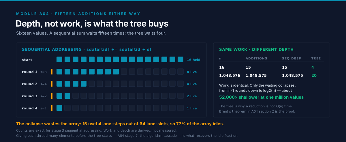
Watch what the rounds do to the array. Half the lanes fall idle at every level, so by the final round one lane in sixteen is still working — only 15 of the 64 lane-slots ever do anything. The depth win is real and it is the reason to use a tree, but the idle fraction is a real bill, and stage 7 below is the rung that pays it off.
The GPU version has three nested levels of this tree, and they are not the same mechanism:
| Level | Span | How values are exchanged | Sync primitive |
|---|---|---|---|
| Warp / wavefront | 32 or 64 lanes | registers, via __shfl_* |
implicit lockstep (AMD) / __syncwarp (NVIDIA Volta+) |
| Block / workgroup | 128–1024 threads | shared memory / LDS | __syncthreads() |
| Grid | all blocks | global memory | second kernel launch, or atomics |
Almost every reduction bug and every reduction optimization lives at one of those three boundaries.
The ladder¶
%%{init: {
  'theme': 'base',
  'themeVariables': {
    'primaryColor': '#F8FAFC',
    'primaryTextColor': '#0F172A',
    'primaryBorderColor': '#0891B2',
    'lineColor': '#64748B',
    'secondaryColor': '#E0F2FE',
    'tertiaryColor': '#EEF2FF',
    'fontFamily': 'Inter, Segoe UI, sans-serif'
  }
}}%%
flowchart TB
  S1["1 interleaved + modulo<br/>problem: warp divergence"]
  S2["2 interleaved + strided index<br/>problem: LDS bank conflicts"]
  S3["3 sequential addressing<br/>problem: half the threads idle"]
  S4["4 first add during load<br/>problem: barrier + guard overhead"]
  S5["5 unroll the last warp<br/>problem: runtime loop bounds"]
  S6["6 complete unroll, templated<br/>problem: too little work per thread"]
  S7["7 grid-stride cascade<br/>now: bandwidth-bound"]
  S8["8 warp shuffle + cascade<br/>same speed, far less LDS"]
  S9["9 shuffle + atomicAdd<br/>one launch, nondeterministic"]

  S1 --> S2 --> S3 --> S4 --> S5 --> S6 --> S7 --> S8 --> S9

  classDef warn fill:#FEF3C7,stroke:#F59E0B,color:#0F172A
  classDef trackA fill:#0891B2,stroke:#0F172A,color:#fff
  classDef success fill:#10B981,stroke:#0F172A,color:#fff
  class S1,S2 warn
  class S3,S4,S5,S6 trackA
  class S7,S8 success
  class S9 warn
Each rung names the problem the next rung solves; the colour change at stage 7 marks where the kernel stops fighting itself and starts being limited only by HBM.
Stage 1 — interleaved addressing with %: warp divergence¶
At s = 1 the active threads are 0, 2, 4, 6, … — every other lane. A warp/wavefront issues one
instruction for all its lanes, so the hardware runs the add with half the lanes masked off. At
s = 2 it is every fourth lane, and so on. There is no step at which a warp is fully busy, and
every warp in the block participates in every step. Two costs, not one:
- Divergence: useful work per issued instruction falls
as
1/(2s). - The
%itself: integer modulo by a runtime value is not a cheap instruction on a GPU. (Had2*sbeen a compile-time power of two the compiler would turn it into a mask; it cannot here.)
Stage 2 — strided index: divergence gone, bank conflicts arrive¶
Now the first blockDim/(2s) threads are the active ones — a contiguous range, so whole warps are
either fully active or fully idle. Divergence is gone. But look at the addresses: consecutive lanes
now touch shared-memory words 0, 2s, 4s, ….
Shared memory (LDS on AMD) is banked: 32 banks of
4-byte words, and a warp can service 32
accesses in one cycle only if they land in 32 distinct banks
(A02 §3). With a stride of 2s words,
lanes collide modulo 32:
step s |
word stride | distinct banks touched by 32 lanes | conflict |
|---|---|---|---|
| 1 | 2 | 16 | 2-way |
| 2 | 4 | 8 | 4-way |
| 4 | 8 | 4 | 8-way |
| 8 | 16 | 2 | 16-way |
| ≥16 | ≥32 | 1 | 32-way |
Each conflict serializes the access. You traded a divergence problem for a memory problem.
Stage 3 — sequential addressing: both problems gone¶
for (unsigned s = blockDim.x / 2; s > 0; s >>= 1) {
    if (tid < s) sdata[tid] += sdata[tid + s];
    __syncthreads();
}
Walk the stride down instead of up. Active threads are always tid < s — contiguous, so no
divergence — and the two operands sdata[tid] and sdata[tid + s] are consecutive words across
lanes, so 32 lanes hit 32 distinct banks. Conflict-free. This addressing pattern is the one that
appears in every production reduction; stages 1 and 2 exist so you understand why.
Stage 4 — first add during the global load¶
Stage 3 has a structural embarrassment: at the very first step only half the threads work, at the second only a quarter, and so on. Over the whole tree, average utilization is barely above one thread. Harris's fix does not touch the loop at all — it changes the launch:
unsigned i = blockIdx.x * (blockDim.x * 2) + threadIdx.x;
float v = (i < n) ? in[i] : 0.0f;
if (i + blockDim.x < n) v += in[i + blockDim.x];   // both loads coalesced
sdata[tid] = v;
Each block now consumes 2 × blockDim.x elements, so you launch half as many blocks, each doing
one extra add during a load it was making anyway. Both loads are coalesced (lane L reads element
base + L and base + blockDim + L). Same total work, half the block-tree overhead. This is the
first hint of the idea that stage 7 takes to its limit.
Stage 5 — unroll the last warp¶
Once s ≤ 32, only one warp is still active. Everything the loop does for those last six steps is
overhead: a barrier that synchronizes 256 threads when 32 are working, and a tid < s guard whose
answer the hardware already knows. So stop the loop at 32 and write the tail straight:
// HIP: safe as written, because AMD guarantees wavefront lanes run in lockstep.
__device__ void warp_tail_volatile(volatile float* s, unsigned tid) {
    s[tid] += s[tid + 32];
    s[tid] += s[tid + 16];
    s[tid] += s[tid + 8];
    s[tid] += s[tid + 4];
    s[tid] += s[tid + 2];
    s[tid] += s[tid + 1];
}
Three things about this famous six-line function, and all three are interview material:
- Why
volatileis mandatory. Without it the compiler is free to keeps[tid]in a register across the six statements and write it back once at the end — at which point the other lanes never see the intermediate values, and the answer is wrong.volatileforces every read and write to actually go to shared memory. - Why it is fragile. The whole trick rests on "lanes of one warp execute in lockstep, so no
barrier is needed." AMD's HIP documentation states that guarantee explicitly for wavefronts.
NVIDIA voided it in Volta: independent thread scheduling means lanes of a warp can have
separate program counters and are not guaranteed to reconverge
(CUDA C++ Programming Guide).
The volatile-only tail is
undefined behavior on Volta and later — it may still work, which is the worst possible failure
mode. NVIDIA's own guidance is to insert
__syncwarp()between the steps or to switch to shuffles. Ourcuda/reduction.cudoes the former; compare it side by side withhip/reduction.cpp— it is the only substantive difference between the two files. - Why the constant is 32 and not
warpSize. On a 64-lane CDNA wavefront, unrolling from 32 is still correct (lanes 0–31 are inside one wavefront), it just leaves thes = 32step running as a full barrier when it did not have to. Unrolling from 64 would be faster on CDNA and wrong on a 32-lane RDNA or NVIDIA part. There is no portable compile-time constant to use: as of ROCm 7.0 HIP'swarpSizeis deliberately notconstexpr(matching CUDA), and__AMDGCN_WAVEFRONT_SIZE__is deprecated. The portable options are (a) hard-code 32 and accept a small loss on wave64, (b) template the kernel on the warp size and pick the instantiation on the host after queryinghipDeviceAttributeWarpSize— the approach HIP's own documentation recommends.
Stage 6 — complete unroll with a templated block size¶
Make the block size a template parameter and the entire tree becomes straight-line code:
template <unsigned BLOCK>
__global__ void reduce6(const float* in, float* out, unsigned n) {
    // ...
    if (BLOCK >= 512) { if (tid < 256) sdata[tid] += sdata[tid + 256]; __syncthreads(); }
    if (BLOCK >= 256) { if (tid < 128) sdata[tid] += sdata[tid + 128]; __syncthreads(); }
    if (BLOCK >= 128) { if (tid <  64) sdata[tid] += sdata[tid +  64]; __syncthreads(); }
    if (tid < 32) warp_tail_volatile(sdata, tid);
}
BLOCK is known at compile time, so every if (BLOCK >= …) is folded away and the loop counter,
its comparison, and its increment disappear. Note carefully where the barriers sit: outside the
tid < … guards. A __syncthreads() that only some threads of a block reach is undefined behavior
and in practice hangs the kernel — see §6.
Stage 7 — the algorithm cascade¶
Recall Brent: T_P ≤ W/P + D. Stages 1–6 have each thread consume one or two elements and then pay
log₂(BLOCK) levels of tree overhead. At N = 2²⁴ with 256-thread blocks that is 32,768 blocks
— 32,768 separate trees, 32,768 sets of barriers, and a second and third kernel launch to combine
them. The overhead is proportional to the number of blocks, and the number of blocks is proportional
to N.
So decouple them. Launch a grid sized to the machine (a few blocks per CU/SM), and have each block stream through as much data as it takes using a grid-stride loop:
float sum = 0.0f;
for (unsigned i = blockIdx.x * (BLOCK * 2) + tid; i < n; i += BLOCK * 2 * gridDim.x) {
    sum += in[i];
    if (i + BLOCK < n) sum += in[i + BLOCK];
}
sdata[tid] = sum;   // one tree per block, no matter how large n is
The serial fold is nearly free — it is a register add per element, with perfectly coalesced loads —
and it collapses N elements down to gridDim.x × BLOCK before a single barrier executes. The tree
overhead becomes O(number of blocks) instead of O(N). This is the rung that reaches peak
bandwidth, and it is why the shallower-tree rungs before it stopped mattering.
Harris's slides derive
the same result from the cost model: keep O(N / log N) threads, each doing
O(log N) serial work.
Stage 8 — warp shuffles: the modern idiom¶
__shfl_down(v, delta, width) lets lane L read lane L + delta's register directly. No shared
memory, no address arithmetic, no barrier:
__device__ float warp_reduce_shfl(float v) {
    for (int off = 16; off > 0; off >>= 1) v += __shfl_down(v, off, 32);
    return v;   // valid in lane 0
}
A whole-block reduction becomes: reduce within each 32-lane group, have one lane per group publish
to a tiny shared array, __syncthreads() once, reduce that array in the first group. One barrier
instead of log₂(BLOCK), and BLOCK/32 floats of LDS instead of BLOCK — which directly buys
occupancy back.
Two portability points that come up constantly:
- Lane count. A NVIDIA warp and an RDNA wavefront are 32 lanes; a CDNA wavefront is 64. The
code above uses
width = 32deliberately: HIP's shufflewidthargument splits the wavefront into independent sub-groups indexed bylaneIdx % width, so a width-32 shuffle behaves identically on wave32 and wave64 hardware. It is the cheapest correct portability strategy; the fully-tuned alternative is to template on the warp size and select at launch. - The
_syncvariants. On CUDA,__shfl_downwas deprecated and replaced by__shfl_down_sync(mask, …)with a 32-bit mask (0xfffffffffor a full warp) — mandatory from Volta onward. HIP added_syncvariants too, but the mask is 64-bit (a wavefront can have 64 lanes), enabled by default from ROCm 7.0. Porting CUDA code that passes0xffffffffto a HIP_syncbuiltin will trip astatic_assert— that is the header protecting you from an implicitly promoted mask, not a bug.
__shfl_down vs __shfl_xor. __shfl_down produces the answer in lane 0 only; the butterfly
form v += __shfl_xor(v, mask, 32) produces it in every lane, for the same instruction count.
Use xor whenever all lanes need the result — softmax
normalization and layer-norm are the standard
examples, since every lane must then divide by the reduced value.
Finishing the job: combining across blocks¶
There is no cheap grid-wide barrier in the base programming model (cooperative groups offer
grid.sync(), at the cost of a launch that must fit entirely on the device at once). Three real
options:
| Strategy | Launches | Deterministic? | When to use |
|---|---|---|---|
| Second kernel on the partials | 2 (or 3) | Yes — fixed partials array, fixed traversal order | Default. Anything feeding training math. |
atomicAdd from each block |
1 | No — block completion order varies | Small N where launch latency dominates, and the consumer tolerates drift |
__threadfence() + last-block-finishes |
1 | Yes, if the last block reads the partials in index order | Single-launch and deterministic, at the cost of a fiddly atomic counter |
The determinism caveat is not pedantry. atomicAdd on floats makes the summation order depend on
how the scheduler happens to retire blocks, and because float addition is not associative, the
same program on the same input can return different low-order bits on every run. In a training
loop that means loss curves that do not reproduce across restarts and "is this diff a regression?"
becoming unanswerable. The main lab measures this directly — see the determinism probe at the end of
its output.
Why every __syncthreads() is required¶
Shared memory is only guaranteed coherent across a block at a barrier. In the tree:
- After the load, before the first step. Thread
tidwritessdata[tid], then readssdata[tid + 128]— a slot owned by a thread in a different wavefront. With 256 threads and 64-lane wavefronts a block is four independently scheduled wavefronts; nothing orders wavefront 3's store before wavefront 0's load. Without the barrier you read uninitialized shared memory. - Between every pair of tree levels. Level
swritessdata[0 … s−1]; levels/2reads them. Same hazard, once per level.
The failure mode is a data race: not a crash, not a consistent wrong answer, but an answer that is sometimes right. Exercise 2 makes you feel it.
And the trap that is worse than forgetting one: putting the barrier inside the divergent branch.
for (unsigned s = BLOCK/2; s > 0; s >>= 1) {
    if (tid < s) { sdata[tid] += sdata[tid + s]; __syncthreads(); }   // UNDEFINED
}
__syncthreads() is a block-wide rendezvous: every non-exited thread of the block must execute it,
and all must execute the same barrier. Wavefronts whose lanes all have tid >= s skip the branch
entirely and never arrive; the ones that did arrive wait forever. On real hardware this hangs
until a watchdog kills the kernel. Barriers belong at uniform control flow — always outside the
if. (Divergent branches are fine; divergent barriers are not.)
4. Hands-On Labs¶
All commands run from this module directory.
# AMD
make hip GPU_ARCH=gfx942     # build hip/ programs
make run-hip                 # run them

# NVIDIA
make cuda SM_ARCH=sm_90      # build cuda/ programs
make run-cuda

# Triton (either vendor)
python triton/reduction.py
The drills are self-contained too: exercises/ and solutions/ each
have their own Makefile, so you can cd exercises && make run without coming back here. From this
directory, make exercises / make solutions build them in place, and make clean cleans all three.
Match
GPU_ARCHto your GPU.gfx950= MI350,gfx942= MI300,gfx90a= MI200,gfx1100= RDNA3. Find yours with/opt/rocm/bin/offload-arch(orrocminfo | grep gfx). Toolchain troubleshooting (missinglibamdhip64.so,hipErrorNoBinaryForGpu) is covered in A01 §4.
Lab 1 — The whole ladder in one table (reduction)¶
Files: hip/reduction.cpp · cuda/reduction.cu.
One program reduces the same 16.7 M-element array nine times, once per rung. For each it prints the time, the effective bandwidth, the speedup over stage 1, the relative error against a float64 CPU reference, and PASSED/FAILED. Output shape:
device          : <your GPU> (<N> CUs/SMs)
n               : 16777216 floats (64.0 MiB), block = 256, cascade grid = <8 x CUs>
reference (fp64): <exact sum>

stage                                                      ms      GB/s    vs #1    rel err  result
---------------------------------------------------- -------- --------- -------- ---------- ------
1 interleaved, modulo branch (divergent)                <...>     <...>    1.00x     <~1e-7> PASSED
...
9 shuffle + atomicAdd (1 launch, nondeterministic)      <...>     <...>    <...>     <~1e-7> PASSED

determinism probe (8 repeats of the same input):
  stage 8 (second kernel launch): bitwise identical every run   [min ..., max ...]
  stage 9 (atomicAdd): results DIFFER between runs              [min ..., max ...]
What to observe — in this order:
- Every stage says PASSED. The ladder is nine implementations of the same function. Nothing in it trades correctness for speed. If a stage fails, that is a real bug, not a rounding effect.
- The relative error column is not zero, and not the same for every stage. Each stage visits the additions in a different order; float addition is not associative. A drift around 1e-7 is the expected signature of a correct float32 tree.
- The jumps, not the absolute numbers. Expect the big steps at stage 3 (divergence and bank conflicts both gone) and stage 7 (enough work per thread to saturate the memory system), and expect stages 7, 8 and 9 to cluster together — once you are bandwidth-bound, further kernel cleverness has nothing left to buy.
- The determinism probe. Stage 8 and stage 9 compute the same sum with the same kernel; only the cross-block combine differs. Stage 8 should be bitwise identical across all eight repeats; stage 9 usually is not.
Absolute times and GB/s are hardware-, driver-, and N-dependent — do not compare your numbers
to anyone else's, compare them to your own machine's copy ceiling
(A02 Lab 1).
Lab 2 — What the compiler already knows (triton/reduction.py)¶
File: triton/reduction.py.
Triton's tl.sum emits the divergence-free, conflict-free, shuffle-based intra-block tree for you —
rungs 1 through 6 of the ladder are simply not decisions you get to make wrong. What Triton does
not decide is the part that actually determines performance: how many elements each program
consumes, and how the partials are combined. So the script benchmarks exactly those, plus
torch.sum as the library baseline.
What to observe: the cascade version should beat the one-program-per-block version and land near
torch.sum — which is itself a tuned cascade. The lesson is not "Triton is fast", it is which
decisions survive the abstraction: the top two rungs of the ladder are yours in every language.
Lab 3 (optional) — Profile it¶
# AMD
make profile-hip     # rocprofv3 summary + traces
# NVIDIA
make profile-cuda    # nsys timeline; then: ncu --set full ./cuda/reduction.exe
What to look for:
- The per-kernel durations confirm the table, and show you the second and third launches that the table folds into one number.
- Nsight Compute's Warp State / branch-efficiency metrics on stage 1 versus stage 3 make the
divergence visible; the Shared Memory section shows bank conflicts on stage 2 dropping to zero
on stage 3. (
rocprofv3exposes the equivalent LDS bank-conflict counter.) - On stages 7–9, look at DRAM throughput as a percentage of peak. That number, not the kernel time, is the one to report in a review.
5. Performance Analysis¶
The only ceiling that matters¶
A reduction reads N values and writes one. There is no reuse, no output traffic to speak of, and
one FLOP per element:
bytes moved      ≈ N * sizeof(float)          (the write is a single scalar)
FLOPs            = N - 1
arithmetic       = (N-1) / (4N) ≈ 0.25 FLOP/byte
effective_GBps   = N * sizeof(float) / kernel_time_seconds
A data-center GPU's roofline ridge point — where memory-bound becomes compute-bound — sits around 30 FLOP/byte (order 10² TFLOP/s ÷ order 10¹² B/s). At 0.25 FLOP/byte a reduction is roughly 120× to the left of the ridge: as memory-bound as a kernel can be.
%%{init: {
  'theme': 'base',
  'themeVariables': {
    'primaryColor': '#F8FAFC',
    'primaryTextColor': '#0F172A',
    'primaryBorderColor': '#0891B2',
    'lineColor': '#64748B',
    'secondaryColor': '#E0F2FE',
    'tertiaryColor': '#EEF2FF',
    'fontFamily': 'Inter, Segoe UI, sans-serif'
  }
}}%%
flowchart LR
  RED["reduction<br/>0.25 FLOP/byte"] -->|"limited by HBM"| BW["Bandwidth ceiling<br/>ridge point ~30 FLOP/byte"]
  VA["vector add<br/>0.08 FLOP/byte"] -->|"limited by HBM"| BW
  GEMM["dense GEMM<br/>10s-100s FLOP/byte"] -->|"limited by FLOP/s"| COMP["Compute ceiling"]

  classDef warn fill:#FEF3C7,stroke:#F59E0B,color:#0F172A
  classDef trackB fill:#6366F1,stroke:#0F172A,color:#fff
  class RED,VA warn
  class GEMM,BW,COMP trackB
Reduction sits next to vector add on the memory-bound side; the practical consequence is that once you reach a high fraction of HBM bandwidth, there is nothing left to optimize in the kernel.
Therefore: the success metric for a reduction is effective_GBps / your measured copy ceiling.
Not the speedup over stage 1, not the instruction count. Get your ceiling from
A02 Lab 1
(hip/bandwidth.exe), and expect a well-tuned reduction to land in the 80–90% range of it.
Expected shape of results¶
We deliberately do not publish a measured table here — the numbers depend on your GPU, driver,
ROCm/CUDA version, and N, and a stale table teaches the wrong thing. Run Lab 1 and fill in your
own. What is reproducible is the ordering and the shape:
| Transition | Why it helps | Expected magnitude |
|---|---|---|
| 1 → 2 | removes warp divergence and the runtime % |
large |
| 2 → 3 | removes shared-memory bank conflicts | large |
| 3 → 4 | halves the block count, one free add per load | moderate |
| 4 → 5 | drops six barriers and six guards per block | moderate |
| 5 → 6 | folds the loop away at compile time | small |
| 6 → 7 | decouples tree overhead from N — the bandwidth rung |
large |
| 7 → 8 | LDS traffic → registers | small (both are bandwidth-bound) |
| 8 → 9 | removes one kernel launch | small, and costs determinism |
Cumulatively this is a large multiple, not a few percent: the original Harris slides report roughly a 30× improvement from kernel 1 to kernel 7 on a 4 M-element reduction (on a G80 — the absolute numbers are of historical interest only; the ordering has held up across twenty years of architectures). The per-stage table is in the deck; reproduce its shape on your own hardware rather than trusting either their numbers or ours.
Reading your own result¶
- Compute
effective_GBpsfor your best stage (the program prints it). - Divide by your measured copy ceiling.
- Above ~80%: you are done. Any further work belongs elsewhere in the pipeline — fuse this reduction into the kernel that produced the data, or stop reducing so often.
- Below ~60%: check, in this order — is
Nlarge enough that launch latency is not dominating (see exercise 3, Q7)? Is each thread loading enough elements to keep requests in flight (try unrolling the grid-stride loop or usingfloat4loads)? Is the grid actually filling the machine?
6. Challenges, Drawbacks & Tradeoffs¶
%%{init: {
  'theme': 'base',
  'themeVariables': {
    'primaryColor': '#F8FAFC',
    'primaryTextColor': '#0F172A',
    'primaryBorderColor': '#0891B2',
    'lineColor': '#64748B',
    'secondaryColor': '#E0F2FE',
    'tertiaryColor': '#EEF2FF',
    'fontFamily': 'Inter, Segoe UI, sans-serif'
  }
}}%%
flowchart TD
  Q{"Reduction misbehaving?"}
  Q -->|"wrong, and differs run to run"| E1["Missing __syncthreads()"]
  Q -->|"kernel hangs"| E2["Barrier inside a divergent branch"]
  Q -->|"wrong only on some GPUs"| E3["Warp-size or lockstep assumption"]
  Q -->|"wrong only for some inputs"| E4["Wrong identity element for the tail"]
  Q -->|"right but not reproducible"| E5["atomicAdd combine, float non-associativity"]
  Q -->|"correct but slow"| E6["Too few elements per thread"]

  E1 --> F1["Barrier after the load and between tree levels"]
  E2 --> F2["Move the barrier to uniform control flow"]
  E3 --> F3["width-32 shuffles, or template on queried warpSize;<br/>__syncwarp on Volta+"]
  E4 --> F4["Identity: 0 for sum, -inf for max, 1 for product"]
  E5 --> F5["Second kernel launch over a fixed partials array"]
  E6 --> F6["Grid-stride cascade; grid sized to the machine"]

  classDef warn fill:#FEF3C7,stroke:#F59E0B,color:#0F172A
  classDef success fill:#10B981,stroke:#0F172A,color:#fff
  class Q,E1,E2,E3,E4,E5,E6 warn
  class F1,F2,F3,F4,F5,F6 success
Six symptoms, six distinct root causes — note that three of them produce a program that passes its tests most of the time.
Pitfall 1 — The missing barrier (silent, intermittent, and the most common)¶
Covered in §3. What makes it dangerous is that it often works: with a small block, or a lucky
schedule, or a debug build, the wavefronts happen not to drift. Do not conclude from a green run
that a barrier was unnecessary. Conclude it from the memory model, and confirm with
compute-sanitizer --tool racecheck.
Pitfall 2 — The divergent barrier (hangs, does not fail)¶
__syncthreads() inside if (tid < s). Whole wavefronts never arrive, the rest wait forever. §3
has the code and the reasoning. The rule to memorize: branch divergently all you like; synchronize
uniformly.
Pitfall 3 — Assuming a warp size, or assuming lockstep¶
Two separate assumptions, both fatal, and both invisible until you change hardware:
- Size. 32 on NVIDIA and RDNA, 64 on CDNA. A hand-unrolled 32-lane tail is correct everywhere
but suboptimal on wave64; a hand-unrolled 64-lane tail is wrong on wave32. HIP's
warpSizeis intentionally not a compile-time constant (as of ROCm 7.0, matching CUDA), and__AMDGCN_WAVEFRONT_SIZE__is deprecated — queryhipDeviceAttributeWarpSizeon the host and dispatch to a templated kernel if you need the last few percent. - Lockstep. AMD guarantees wavefront lanes execute in lockstep. NVIDIA does not, since Volta
introduced independent thread scheduling. Warp-synchronous code that omits
__syncwarp()or the_syncshuffle variants is undefined behavior on modern NVIDIA parts.
Pitfall 4 — The identity element for partial tiles¶
N is almost never an exact multiple of the tile size, so some lanes have no data and must
contribute the operator's identity: 0 for sum, 1 for product, −∞ for max, +∞ for min,
false for logical-or. Using 0.0f as the identity for a max reduction is the classic version
of this bug, and it is invisible until someone feeds you an all-negative array. That is exercise 1.
Pitfall 5 — Determinism, and why ML cares¶
Float addition is not associative: (a+b)+c ≠ a+(b+c) in general. Consequences, in increasing order
of how much trouble they cause:
- Across implementations. The nine ladder stages produce nine slightly different answers to the same question. All are equally "correct"; none matches a sequential CPU sum exactly. Always verify against a float64 reference with a tolerance, never against a float32 sequential loop.
- Across runs. Only the atomic-combine variant has this problem, and it is a real one. A gradient norm that changes in its last bits changes the clipping scale, which changes the update, which — after enough steps — changes the model. Debugging "my run diverged and I cannot reproduce it" is expensive; a deterministic second launch costs microseconds.
- Precision loss. A long sequential float32 sum stagnates: once the running total is large
enough, adding a small value rounds to no change. The tree is actually better here — its error
grows like
O(log N)rather thanO(N)— which is a rare case where the parallel algorithm is also the more accurate one. Where accuracy really matters, accumulate in float64 or use a compensated (Kahan) sum (Goldberg, 1991), and accept the cost.
Pitfall 6 — Reducing when you should not be reducing¶
The reduction itself is cheap; launching it is not. Below roughly ten million elements the two
kernel launches cost as much as moving the data (exercise 3 works the number out). In a training
loop, where you reduce a scalar loss or a per-layer gradient norm thousands of times per step, the
answer is never "write a faster reduction kernel" — it is fuse the reduction into the kernel that
produced the data, batch many small reductions into one launch, capture the sequence in a
CUDA/HIP graph, and above all do not call .item() inside the loop.
Tradeoffs to hold in mind¶
- Second launch vs atomics: determinism and a partials buffer, versus one fewer launch. Default to the launch; deviate only with a reason you would write in a code review.
- Shared memory vs shuffles: shuffles use fewer barriers and less LDS (better occupancy) but only work within a warp, so you always need some shared memory for the block level.
- Hand-written vs library: rocPRIM / hipCUB / CUB / Thrust already implement everything in this
module, tuned per architecture, and
torch.sumcalls into them. Write your own when you need to fuse the reduction with surrounding work (that is the real win) — not to beat the library at the standalone operation, because you will not.
7. Real-World Use Cases¶
Reduction is not a teaching toy; it is arguably the second most executed pattern in machine learning after GEMM. Everywhere a tensor becomes a scalar (or a smaller tensor), this is the kernel.
- The loss itself.
loss = criterion(pred, target)ends in ameanorsumover the batch — a reduction to a single scalar, run every forward pass. Andloss.item()is the single most common accidental pipeline stall in PyTorch training loops, precisely because it forces a synchronization on the result of this reduction. torch.sum/torch.mean/torch.max/torch.norm. All of these dispatch to a tuned cascade reduction in ATen, backed by CUB (CUDA) or hipCUB/rocPRIM (ROCm). Everydim=argument variant is the same ladder with a different mapping of threads to the reduced axis; reducing along the contiguous axis is the coalesced case, reducing across it is the transpose problem from A02 in disguise.- Gradient norms for clipping.
clip_grad_norm_computessqrt(Σ ‖g‖²)over every parameter tensor in the model — thousands of small reductions per optimizer step. This is exactly the "many small reductions" case of §6 pitfall 6, which is why PyTorch shipstorch._foreach_norm: one fused launch instead of thousands. It is also the place where the atomics-determinism issue bites hardest, since the clipping scale feeds directly into the weight update. - Softmax denominators.
softmax(x)ᵢ = exp(xᵢ − max(x)) / Σⱼ exp(xⱼ − max(x))needs two reductions per row — a max (for numerical stability) and a sum. Every lane needs both results, so this is the canonical__shfl_xorbutterfly case. FlashAttention's central trick is a running (online) version of these two reductions so the softmax never needs the full row in memory at once — the reduction pattern is the load-bearing part of the algorithm. - Normalization layers. BatchNorm, LayerNorm, RMSNorm and GroupNorm all compute mean and variance over some axis — two reductions (or one, using the sum/sum-of-squares trick, which is faster and numerically worse). Because these run per layer per step, their launch overhead is a measurable fraction of training time, which is why every framework fuses them.
- Distributed training: allreduce.
torch.distributed.all_reduce, NCCL and RCCL implement the same algorithm one level up the hierarchy — ring and tree allreduce are literally a reduction where the "lanes" are GPUs and the "shared memory" is the interconnect (Infinity Fabric, NVLink, InfiniBand). Data-parallel training performs one allreduce over the entire gradient buffer every step, and the same three questions apply: what is the tree shape, where are the barriers, and is the result bit-reproducible across runs? - Everything else that produces a metric. Accuracy counts, token counts, histogram bins, loss
scaling factors for mixed precision (which reduce over "did any gradient overflow?" — a logical-or
reduction, identity
false).
Libraries that embody this module: rocPRIM / hipCUB (AMD), CUB / Thrust (NVIDIA),
RCCL / NCCL for the multi-GPU version, and every tl.sum in a Triton kernel you will write in
A08.
Where to go next. A05 asks the same tree for every prefix rather than just the total, which is where the work-efficiency §2 got for free turns into an explicit choice. A07 is the payoff §6 keeps pointing at: two of these reductions per row, folded into the operator that produced the data instead of launched after it. B03 turns Lab 3 from a sanity check into a method — divergence, bank-conflict and DRAM-throughput counters are how you prove which rung a kernel is standing on instead of inferring it from the clock.
8. Cited References¶
Sources shared with other modules are cited by anchor into the master bibliography, where the URL and its retrieval date live. The last five are used only by this module, so they carry their citation in full.
- Optimizing Parallel Reduction in CUDA (Harris) — the ladder §3 rebuilds rung by rung, the cost model behind the stage-7 cascade, and the source of the historical 30× figure quoted in §5.
- CUDA C++ Programming Guide
— the normative statement of
__syncthreads()semantics, warp-level primitives, and the independent thread scheduling that makes §3 stage 5's volatile-only warp tail undefined behavior on Volta and later. - CUDA C++ Best Practices Guide — shared-memory bank conflicts (the stage-2 table), occupancy, event timing, and the effective-bandwidth definition §5 measures against.
- HIP Programming Model — the AMD
spelling of the three-level hierarchy in §3: wavefronts, workgroups, LDS,
__syncthreads(). - Roofline (Williams et al., 2009) — why 0.25 FLOP/byte settles the question of what a reduction can possibly be limited by, and therefore why §5 reports a fraction of peak bandwidth rather than a speedup.
- What Every Computer Scientist Should Know About Floating-Point Arithmetic (Goldberg, 1991) — non-associativity, absorption in a long running sum, and compensated summation: the arithmetic behind §2's caveat and §6 pitfall 5.
- Lin, Y. & Grover, V. Using CUDA Warp-Level Primitives (NVIDIA blog) — why the volatile-only
warp tail is unsafe on Volta+, and the
__syncwarp()/__shfl_*_syncreplacements. Retrieved 8 Aug 2026. https://developer.nvidia.com/blog/using-cuda-warp-level-primitives/ - HIP C++ Language Extensions —
warpSizesemantics (not a compile-time constant), wavefront lockstep guarantee, shufflewidthsub-groups, the 64-bit_syncmask. Retrieved 8 Aug 2026. https://rocm.docs.amd.com/projects/HIP/en/latest/how-to/hip_cpp_language_extensions.html - rocPRIM — AMD's production reduction/scan primitives; what to use instead of hand-rolling. Retrieved 8 Aug 2026. https://rocm.docs.amd.com/projects/rocPRIM/en/latest/
- Brent, R. P. (1974). The Parallel Evaluation of General Arithmetic Expressions, JACM 21(2) —
the
T_P ≤ W/P + Dbound used in §2. https://dl.acm.org/doi/10.1145/321812.321815 - Higham, N. J. (1993). The Accuracy of Floating Point Summation, SIAM J. Sci. Comput. 14(4) —
the
O(log N)vsO(N)error growth claim in §6. https://epubs.siam.org/doi/10.1137/0914050
9. Self-Assessment & Interview Drills¶
Conceptual (answers below)¶
- A reduction over
Nelements has workW = N−1and depthD = log₂N. Your GPU has ~10⁵ concurrent lanes andN = 2²⁴. Using Brent's bound, which term dominates — and what does that tell you about which optimizations are worth doing? - Stage 1 uses
if (tid % (2*s) == 0)and stage 2 usesindex = 2*s*tid. Both compute the same tree. Name the problem each one has, and explain why fixing the first created the second. - Why is
volatilerequired in the classic unrolled warp tail, and why is that same code undefined behavior on an NVIDIA Volta or newer GPU? Give both fixes. - You hand-unroll the last 64 lanes because your MI300X has 64-lane wavefronts. What breaks, and on what hardware? What is the portable way to get the same win?
- A colleague moves
__syncthreads()insideif (tid < s)"so idle threads don't waste time at the barrier." What happens, and why is it worse than the original? - Your reduction returns a slightly different value on every run. The code has no race and passes
racecheck. What is the most likely cause, and what would you change if the value feeds gradient clipping? - Convert a sum reduction to a max reduction. Which single line is most likely to be wrong, and which input exposes it?
- Explain to a non-programmer, in two sentences, why adding up a million numbers on 1000 workers is not 1000× faster than one worker.
Answers
W/P = 16,777,215 / 100,000 ≈ 168versusD = 24— the work term dominates by ~7×. Therefore optimizations that reduce depth (a shallower tree) are nearly worthless, while optimizations that raise effective throughput per lane (removing divergence, removing bank conflicts, giving each thread more elements) are where all the gains are. This is precisely why the ladder's two biggest rungs are stage 3 and stage 7.- Stage 1's active lanes are scattered (
0, 2, 4, …), so the warp executes every step with most lanes masked off — warp divergence — and pays a runtime integer modulo. Stage 2 makes the active lanes contiguous (the firstblockDim/2sthreads), which kills divergence, but their shared-memory addresses now stride by2swords, which collides in the 32 LDS banks: a 2-way conflict ats=1growing to 32-way. Fixing the lane mapping changed the address mapping; stage 3's downward stride is the pattern that satisfies both constraints at once. volatileprevents the compiler from cachings[tid]in a register across the six statements and writing back only at the end, which would hide the intermediate values from the other lanes. It is UB on Volta+ because independent thread scheduling removed the guarantee that warp lanes execute in lockstep and reconverge —volatileorders the compiler, not the hardware. Fixes: insert__syncwarp()between the steps (keeping the shared-memory tail), or replace the whole tail with__shfl_down_syncregister shuffles. The shuffle version is preferred: it is faster, uses no shared memory, and has no volatile sharp edges.- It is wrong on any 32-lane device — NVIDIA (all of them) and AMD RDNA (gfx10/gfx11). Lanes 32–63
are a different wavefront there, so reading
s[tid+32]without a barrier is a cross-wavefront race. Portable win: template the kernel on the warp size, queryhipDeviceAttributeWarpSize(orcudaDeviceProp::warpSize) on the host, and launch the matching instantiation. Cheaper approximation: usewidth = 32shuffle sub-groups, which behave identically on wave32 and wave64 (this module's approach). - Whole wavefronts whose lanes all have
tid >= snever execute that barrier, so the wavefronts that did arrive wait for participants who will never come — the kernel hangs until a watchdog kills it. It is worse than the original because a hang gives no answer at all and no stack trace, whereas a missing barrier at least produces output you can compare.__syncthreads()must be reached by every non-exited thread of the block; branch divergently, synchronize uniformly. - Almost certainly an
atomicAdd-based cross-block combine: block completion order varies with scheduling, and float addition is not associative, so the summation order — and therefore the low bits — changes run to run. For a gradient norm, switch to a deterministic second kernel launch over a fixed partials array (or the__threadfencelast-block pattern). The few microseconds are worth reproducible training. - The identity element — the value assigned to lanes with no data.
0.0fis right for sum and catastrophically wrong for max, because it beats every negative input. The exposing input is an array whose true maximum is negative, with a length that is not a multiple of the tile size (so that some lanes really are idle). Correct identity:-INFINITY(or-FLT_MAXif a downstream consumer cannot handle infinities). - Splitting the work means every worker has to hand their partial answer to someone else, and those hand-offs cost time that a single worker never pays. You also cannot start combining until enough workers have finished, so the slowest one sets the pace — with a million numbers the split is still a huge win, but with a hundred the hand-offs cost more than just adding them yourself.
Coding & Algorithms drills¶
Do these in exercises/; reference answers in solutions/. Write real,
compiling, edge-case-correct code — no pseudo-code. Expected terminal output (PASS and the
instructive FAIL states) is in
exercises/README.md → Sample sandbox output.
- Max reduction (
exercises/01_max_reduce.cpp) — re-target the sum reduction tomax. Two TODOs: the operator, and the identity element for lanes with no data. Three test cases; the all-negative one with a non-multiple length is the one that catches a wrong identity, and the single-element one shows why small tests can't distinguish operators. - Find the missing barriers (
exercises/02_fix_sync.cpp) — a block reduction with two absent__syncthreads()calls produces wrong and/or nondeterministic results across 20 repeats. Diagnose from the memory model, fix, and confirm the run-to-run stability. The header also documents the divergent-barrier trap that hangs rather than failing. - Reduction roofline drill (
exercises/03_reduction_analysis.md) — givenN, peak bandwidth, and a measured time, compute the theoretical floor, the fraction of peak achieved, where the remaining gap goes, and at whatNlaunch overhead takes over. Ends with a code-review call on the atomics-versus-determinism tradeoff.
Stretch¶
- Butterfly reduction. Rewrite the warp step with
__shfl_xorso every lane ends with the total, then use it to write a single-pass row-softmax (max and sum in one kernel). Compare againsttorch.softmax. - Beat your own stage 7. Add
float4vectorized loads to the grid-stride loop and re-measure. Predict the gain from the memory-level-parallelism argument in §5 before you run it. - Deterministic single launch. Implement the
__threadfence()+ atomic-counter "last block finishes" pattern, and prove with the determinism probe that it is bitwise stable across runs while still using only one launch. - Segmented reduction. Reduce 10,000 independent rows of 512 elements each in one launch (one
block per row), and compare against 10,000 separate small reductions. This is the
torch._foreach_normproblem from §7.