B07 — Distributed Training & Sharding¶
Track B · Module 07 · Status: DONE · Est. 8 hours · Depth 4/5
Prerequisites: A01 (kernels, host/device model), A04 (reduction — and its floating-point associativity warning), and B01 for the interconnect hierarchy, whose §3.5 measures the links this module spends: 7 × 128 GB/s bidirectional Infinity Fabric per MI300X (896 GB/s aggregate) against 5.3 TB/s of HBM — a ~6× gap that is the reason everything below exists. Helpful: B05 (transformer shapes), B06 (serving and the KV cache). This module derives what it needs so it stands alone, and builds on B01's link arithmetic rather than repeating it.
Backends: none. All three tools in
tools/are pure-Python analytic models — no GPU, notorch, nonumpy. You can do this entire module on a laptop, and you should: the point is to make the go/no-go decision before you ask for 512 GPUs. Setup: SETUP.md · Terms: GLOSSARY.md · Sources: REFERENCES.md.
1. TL;DR + Layman analogy¶
TL;DR. A modern model does not fit on one GPU, and the reason is arithmetic you can do in your head: mixed-precision Adam costs 16 bytes per parameter of resident state before a single activation exists, so a 70-billion-parameter model needs ~1043 GiB of state on hardware that has 192 GiB per device. So you shard, and there are exactly four axes to shard along — data (split the batch), ZeRO/FSDP (split the optimizer state, gradients, then parameters), tensor (split individual matrices), and pipeline (split the layers) — plus two specialised ones, expert (MoE) and sequence/context. Each axis trades memory for a different collective communication pattern, and every collective runs on a bandwidth hierarchy that spans three orders of magnitude from intra-node links to the data-centre network. Choosing a parallelism strategy is choosing which communication pattern you can afford where. Real systems nest three or four axes at once, and the nesting order follows directly from that bandwidth hierarchy.
Layman analogy — a construction company building one enormous housing project.
- Data parallel is several identical crews building identical houses on separate lots. Each crew works from the same blueprint, discovers its own set of small corrections during the day, and every evening all crews get on a call and agree on one merged set of blueprint edits before tomorrow. That evening call is an all-reduce. It is simple and it scales beautifully — as long as one crew can hold the whole blueprint and all its tools.
- ZeRO / FSDP is the same crews, but now the tool library is split between them: crew 3 physically stores the plumbing tools, crew 7 the electrical ones. When you need to plumb a wall, you radio for the plumbing tools, use them, and give them straight back. Nobody stores everything, so each crew's shed is far smaller — you just spend the day radioing for tools. That is all-gather just in time.
- Tensor parallel is several workers on the same wall. Worker A lays the left half of every brick course, worker B the right half — so after every single course they must compare edges and agree. They finish the wall much faster, but only if they can literally shout to each other. Put them on radios across town and they will finish slower than one worker alone. This is why tensor parallelism lives inside a node, on NVLink or Infinity Fabric.
- Pipeline parallel is an assembly line: framers, then electricians, then drywall, then painters. The electricians sit idle until the framers finish the first house, and the framers sit idle at the end while the painters catch up. That idle time is the bubble, and the fix is to keep many houses in flight at once (micro-batching) so everybody is busy in the middle.
- Expert parallel (MoE) is specialist subcontractors: each house needs only two of the twelve specialists, but you don't know which two until you inspect it, so every house gets trucked to whichever yards it needs. That routing traffic is an all-to-all, and a day when everyone needs the same specialist is a day that specialist becomes the bottleneck.
Where the analogy breaks — three places, all load-bearing:
- Crews can tolerate disagreement; gradients cannot. Two crews whose walls differ by a millimetre still produce two fine houses. Two data-parallel ranks whose parameters differ produce a divergent model. Synchronisation here is a correctness requirement, not a coordination nicety — and because floating-point addition is not associative, even a correct all-reduce that sums in a different order gives a slightly different answer (A04 §Pitfall 5 makes this precise). Bit-exact reproducibility across a reconfigured cluster is something you choose to pay for, not something you get.
- The analogy has no bandwidth hierarchy. In real hardware, "shouting across the wall" (intra-node, hundreds of GB/s), "radioing the next site" (inter-node, tens of GB/s), and "posting a letter" differ by 10–100×. That single ratio is what decides the entire parallelism layout.
- The slowest crew sets everyone's pace. A synchronous training step ends when the last rank arrives at the barrier, so one GPU that is 10% slow makes 1024 GPUs 10% slow. Section 6 does the statistics of that.
%%{init: {
  'theme': 'base',
  'themeVariables': {
    'primaryColor': '#F8FAFC',
    'primaryTextColor': '#0F172A',
    'primaryBorderColor': '#0891B2',
    'lineColor': '#64748B',
    'secondaryColor': '#E0F2FE',
    'tertiaryColor': '#EEF2FF',
    'fontFamily': 'Inter, Segoe UI, sans-serif'
  }
}}%%
flowchart TB
  ROOT["What do you split?"]

  ROOT --> DP["Data parallel (DDP)<br/>split: the BATCH<br/>replicate: everything else"]
  ROOT --> ZR["ZeRO / FSDP<br/>split: optimizer -> grads -> params<br/>replicate: nothing (stage 3)"]
  ROOT --> TP["Tensor parallel<br/>split: each WEIGHT MATRIX<br/>replicate: the batch"]
  ROOT --> PP["Pipeline parallel<br/>split: the LAYERS<br/>replicate: nothing"]
  ROOT --> EP["Expert parallel (MoE)<br/>split: the EXPERTS<br/>replicate: the router"]
  ROOT --> SP["Sequence / context parallel<br/>split: the SEQUENCE<br/>replicate: the weights"]

  DP --> DPC["communicates: gradients<br/>all-reduce, once per step"]
  ZR --> ZRC["communicates: parameters + gradients<br/>all-gather + reduce-scatter, per layer"]
  TP --> TPC["communicates: ACTIVATIONS<br/>all-reduce, ~4x per layer"]
  PP --> PPC["communicates: stage boundary tensors<br/>point-to-point, 2x per stage"]
  EP --> EPC["communicates: routed tokens<br/>all-to-all, 2x per MoE layer"]
  SP --> SPC["communicates: K/V or partial attention<br/>ring / all-gather, per attention"]

  DPC --> DPF["fails when: model does not fit"]
  ZRC --> ZRF["fails when: comm cannot overlap compute"]
  TPC --> TPF["fails when: link is slow (cross-node)"]
  PPC --> PPF["fails when: too few micro-batches (bubble)"]
  EPC --> EPF["fails when: routing is imbalanced"]
  SPC --> SPF["fails when: sequence too short to pay for it"]

  classDef trackB fill:#6366F1,stroke:#0F172A,color:#fff
  classDef neutral fill:#F8FAFC,stroke:#0891B2,color:#0F172A
  classDef warn fill:#FEF3C7,stroke:#F59E0B,color:#0F172A
  class ROOT neutral
  class DP,ZR,TP,PP,EP,SP trackB
  class DPC,ZRC,TPC,PPC,EPC,SPC neutral
  class DPF,ZRF,TPF,PPF,EPF,SPF warn
Read this diagram as the module's index: every axis is defined by the triple what it splits → what it must communicate → what makes it fail. If you can reconstruct that triple for all six axes from memory, you can pass any distributed-training interview.
By the end of this module you can: compute a training memory budget per GPU from parameters, optimizer, and activations; derive the ring all-reduce cost model and say whether a given collective is latency- or bandwidth-bound; derive the pipeline bubble fraction and the micro-batch count needed to hide it; choose and justify a parallelism combination for a given model, cluster, and interconnect; and name the failure mode each axis brings with it.
2. First Principles¶
2.1 Why you must shard at all: do the memory arithmetic¶
Start with the thing everyone forgets: the parameters are the small part.
Mixed-precision training with Adam keeps five tensors per weight. Walk through why each one has to exist:
| Tensor | dtype | bytes/param | Why it cannot be dropped |
|---|---|---|---|
| Parameter (compute copy) | bf16 | 2 | What the matmuls actually read |
| Gradient | bf16 | 2 | Produced by backward, consumed by the optimizer |
| Master weight | fp32 | 4 | bf16 has ~8 mantissa bits; small updates would round to zero |
Adam first moment m |
fp32 | 4 | Momentum — Adam's whole point |
Adam second moment v |
fp32 | 4 | Per-parameter scaling — Adam's other whole point |
| Total | 16 |
This is the 16 bytes per parameter figure from the
ZeRO paper
(arXiv:1910.02054, which writes it as
2Ψ + 2Ψ + KΨ with K = 12 for Adam). Note that plain fp32 + Adam is also 16
bytes/param (4+4+4+4) — mixed precision
buys you speed and activation memory, not state memory.
Concrete model that cannot fit. Take a Llama-2-70B-shaped model
(arXiv:2307.09288): Ψ = 70e9, L = 80
layers, hidden h = 8192, a = 64 heads, sequence s = 4096.
An MI300X has 192 GB of HBM3; an
H100 SXM has 80 GB. So the state alone
needs 1043 / 192 = 5.4 MI300X-class GPUs, and you have not yet stored a single
activation. Data parallelism cannot help you here — DDP replicates all 1043 GiB on
every rank. This is the entire reason sharding exists.
2.2 Activations: the term that scales with your batch and your context¶
Activation memory is what backward needs from forward. For one transformer layer with 2-byte activations, Megatron's accounting (arXiv:2205.05198, eq. 1) is:
The 34 covers the linear projections, LayerNorms, GeLU, and dropout masks. The
5*a*s/h term is the
attention score matrix,
and it is quadratic in sequence
length — that is the term that kills long-context training.
Apply it to our 70B at s=4096, b=1, h=8192, a=64:
5*a*s/h        = 5 * 64 * 4096 / 8192          = 160
per layer      = 4096 * 1 * 8192 * (34 + 160)  = 6.51e9 bytes = 6.06 GiB
all 80 layers  = 80 * 6.06                     = 485 GiB
485 GiB of activations for a micro-batch of one. Add the state:
   1043 GiB   state (params + grads + optimizer)
+   485 GiB   activations (micro-batch 1, seq 4096)
+    10 GiB   framework/fragmentation reserve
= 1538 GiB per GPU needed   vs   192 GiB available   ->   8.0x over budget
per-GPU HBM budget, 70B model, micro-batch 1, seq 4096   (analytic)

 0 GiB                                                          1538 GiB
 |----------------------------------------|--------------------|--|
 |<------------ state 1043 -------------->|<-- activ 485 ----->|res|
 |==== 192 GiB of MI300X HBM ====|
 ^ you are here                  ^ ...and the model is here
2.3 Activation checkpointing: buy memory with FLOPs¶
If you do not store the activations, you must recompute them. Store only each layer's input and re-run its forward pass during backward (arXiv:1604.06174):
full recompute = 2*s*b*h per layer = 2 * 4096 * 8192 = 67.1 MB/layer
all 80 layers  = 5.4e9 bytes = 5.0 GiB          (was 485 GiB -> 97x less)
The price, derived: a weight matmul costs 2*P*T FLOPs forward and 4*P*T
backward (one matmul for the input gradient, one for the weight gradient), so
forward is 2/6 = 1/3 of the step. Recomputing the whole forward pass adds
another 2*P*T:
Published measurement, attributed: Korthikanti et al. report 42.1% Model
FLOPs Utilization with full activation recomputation vs 54.2% without for a 530B
GPT-style model on 2240 A100s — a 29% throughput difference
(arXiv:2205.05198). Their selective
recomputation targets only the quadratic attention term, leaving 34*s*b*h/t per
layer and costing just 2.7% extra FLOPs for GPT-3. That is why selective
recomputation is the modern default.
Verify all of the above with the planner:
model      : 70.0B params, L=80, h=8192, heads=64
step shape : seq=4096, micro-batch=1, recompute=none
cluster    : 8 GPUs x 192 GiB (reserve 10 GiB, usable 182 GiB)
state      : 2+2+12 = 16 bytes/param -> 1043 GiB unsharded (5.4 GPUs of pure state)

strategy                        axes                      state    activ  reserve    total  fits 192 GiB?
---------------------------------------------------------------------------------------------------------
DDP (replicate everything)      dp=8 tp=1 pp=1 z0        1043.1    485.0     10.0   1538.1  NO
ZeRO-1 (shard optimizer)        dp=8 tp=1 pp=1 z1         358.6    485.0     10.0    853.6  NO
ZeRO-2 (+ shard grads)          dp=8 tp=1 pp=1 z2         244.5    485.0     10.0    739.5  NO
ZeRO-3 / FSDP (+ shard params)  dp=8 tp=1 pp=1 z3         133.6    485.0     10.0    628.6  NO
Tensor parallel tp=8            dp=1 tp=8 pp=1 z0         130.4     60.6     10.0    201.0  NO
Pipeline parallel pp=8          dp=1 tp=1 pp=8 z0         130.4    485.0     10.0    625.4  NO
---------------------------------------------------------------------------------------------------------
all figures GiB per GPU, analytic model (not measured)
Three lessons are visible in that table before you read another word of theory:
- No single axis saves you. Even ZeRO-3 across 8 GPUs leaves 628 GiB/GPU, because it does not touch the 485 GiB of activations.
- Only tensor parallelism shrinks activations (60.6 GiB here), because it is the only axis that splits the tensors inside a layer.
- Pipeline parallelism does not reduce activation memory. Look again:
pp=8still shows 485 GiB. Section 3.4 derives why.
2.4 Collectives are the primitives¶
Every parallelism axis is built from five collective operations. Learn these five and the rest is bookkeeping.
| Collective | What each rank ends up with | Used by |
|---|---|---|
| all-reduce | The sum (or max/avg) of all ranks' buffers, everywhere | DDP gradients, tensor-parallel activations |
| reduce-scatter | Rank i gets the reduced slice i |
ZeRO-2/3 gradients, sequence parallel |
| all-gather | Every rank gets the concatenation of all slices | ZeRO-3 parameters, sequence parallel |
| all-to-all | Rank i sends slice j to rank j — a transpose |
MoE expert routing |
| broadcast | One rank's buffer, copied to all | Initial weights, checkpoint restore |
The identity worth memorising: all-reduce = reduce-scatter + all-gather.
That is not a curiosity — it is why ZeRO-2 gets its memory saving for free
(it was already doing both halves) and why sequence parallelism can replace an
all-reduce with reduce-scatter + all-gather at identical volume.
AMD ships RCCL; NVIDIA ships
NCCL.
RCCL is API-compatible with NCCL, so PyTorch's dist.init_process_group("nccl")
maps onto RCCL on a ROCm build. Both implement ring and tree algorithms and pick
between them by message size and topology.
2.5 Derive the ring all-reduce cost model¶
This is the single most useful formula in distributed training, so derive it, do not memorise it.
Arrange P ranks in a logical ring. Split each rank's S-byte buffer into P
chunks of S/P bytes.
Phase 1 — reduce-scatter (P-1 steps). In each step every rank sends one
chunk to its right neighbour and adds the chunk it receives from its left. After
P-1 steps, rank i holds the fully reduced chunk i. Bytes sent per rank:
(P-1) * S/P.
Phase 2 — all-gather (P-1 steps). Now circulate those finished chunks the
same way, without reducing. Bytes sent per rank: another (P-1) * S/P.
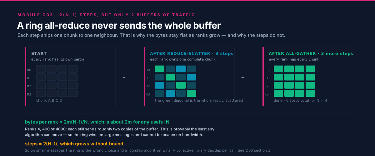
The three panels are the same four ranks at the start, after reduce-scatter, and after all-gather — the shading tracks which chunks are fully reduced, which is the part the formula below is counting.
bytes moved per rank = 2 * (P-1)/P * S            <-- the key result
time  T(S,P)         = 2*(P-1)*alpha  +  (2*(P-1)/P) * S/B
                       \___latency___/    \____bandwidth____/
with alpha = per-step latency and B = achievable per-link
bandwidth. Two
consequences that people get wrong constantly:
- As
Pgrows, the volume converges to2S, notP*S.2(P-1)/P → 2. A large-message ring all-reduce over 1024 ranks moves barely more data per rank than over 8. Ring all-reduce is bandwidth-bound and essentially independent of rank count — this is exactly why it replaced parameter servers (Horovod, arXiv:1802.05799, building on Baidu's ring all-reduce). - Small messages are a different world. The latency term
2(P-1)*alphascales linearly withPand does not care about size at all.
Where is the crossover? Set the two terms equal:
2*(P-1)*alpha = (2*(P-1)/P) * S/B
        alpha = S / (P*B)
           S* = P * alpha * B          <-- latency/bandwidth crossover
Beautifully simple, and it holds for reduce-scatter and all-gather too (the ring
depth cancels). Concretely, for P = 8, alpha = 8 us, B = 50 GB/s:
Below ~3 MiB you are paying for launches, not for wire. This is why gradient
bucketing exists: a 70B model has thousands of individual parameter tensors,
many of them under 1 MiB, and all-reducing each one separately would spend all its
time in latency. Fuse them into buckets larger than S* and the same bytes cost
almost nothing extra. PyTorch DDP's default bucket is 25 MB — comfortably above
S* for typical clusters, which is not a coincidence.
op=allreduce  ranks=8  link=50 GB/s  alpha=8 us
latency/bandwidth crossover S* = P*alpha*B = 3.05 MiB (below this, fuse your messages)

  size MiB   time ms  latency %  busbw GB/s  regime
--------------------------------------------------------------
      0.25     0.121       92.4         3.8  latency-bound
      1.00     0.149       75.3        12.3  latency-bound
      4.00     0.259       43.3        28.4  bandwidth-bound
     16.00     0.699       16.0        42.0  bandwidth-bound
     64.00     2.461        4.6        47.7  bandwidth-bound
    256.00     9.507        1.2        49.4  bandwidth-bound
   1024.00    37.693        0.3        49.9  bandwidth-bound
--------------------------------------------------------------
analytic ring model, not measured
The busbw column is the NCCL/RCCL "bus bandwidth" convention: algorithm
bandwidth S/T scaled by the ring factor 2(P-1)/P, so you can compare it
against the raw link speed. At 0.25 MiB you achieve 3.8 GB/s on a 50 GB/s link —
7% efficiency, purely from launch overhead.
[!NOTE] Honesty about the model, and what
--bwmeans.
- This is a ring-only model. Below the crossover, real NCCL/RCCL switch to tree or one-shot algorithms and beat the ring substantially, so the tool overstates small-message cost. Treat the ring numbers as an upper bound for small messages and a good estimate for large ones, and get the truth from
rccl-tests/nccl-testson your actual fabric.--bwis the bandwidth one rank can drive into the collective, not a single wire's rate. B01 §3.5 pins the hardware down: an MI300X has 7 Infinity Fabric links at 128 GB/s bidirectional, i.e. ~64 GB/s per direction per link, and 896 GB/s aggregate (AMD Instinct cluster design reference). A single-ring collective would use one link (~64 GB/s each way); real libraries run several rings concurrently across all 7 links, which is why a few hundred GB/s is the right order for an intra-node 8-GPU group and why this module uses 300 GB/s as its intra-node figure and 25–50 GB/s across nodes. Do not quote the 896 GB/s aggregate as--bw— that is B01's "most common interconnect arithmetic error."
3. Deep Dive¶
3.1 Data parallel (DDP) — replicate the model, split the batch¶
Mechanism. Every rank holds a full copy of the model and optimizer. Each rank runs forward and backward on its own slice of the global batch, producing a full gradient. One all-reduce averages the gradients so every rank applies an identical update and the replicas stay in lockstep.
Communication volume per step: 2Ψ bytes moved per rank (the 2(P-1)/P ≈ 2
factor times the Ψ-element gradient buffer), independent of rank count.
Why it is still the default. The all-reduce for layer i's gradients can start
as soon as layer i's backward finishes, while layer i-1 is still computing.
With bucketing, communication hides almost entirely behind the backward pass — a
well-tuned DDP job can be ~90% efficient at hundreds of ranks.
That overlap is a claim about two things happening at the same instant, which a flowchart cannot express because it has no time axis:
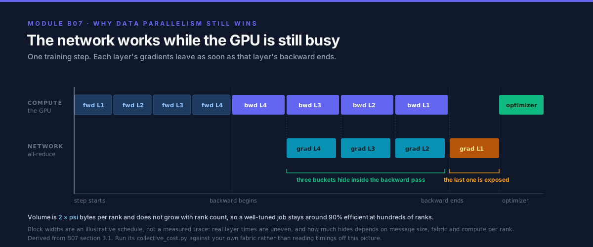
Note the tail. When the final bucket is handed over there is no backward left to cover it, so some exposure is structural rather than a tuning failure — which is why "~90%" and not "100%".
When it wins: the model fits on one device and you want more throughput. Failure mode: the model does not fit — full stop. Also, scaling data parallelism means growing the global batch, and past some critical batch size you get fewer optimizer steps for the same tokens and convergence suffers. Data parallelism is bounded by statistics, not just by hardware.
3.2 ZeRO / FSDP — shard the state, all-gather just in time¶
The insight of ZeRO (arXiv:1910.02054) is that DDP's replication of state is pure waste: every rank stores 16 bytes/param but only needs a given parameter for the microseconds it is being used.
| Stage | Shards | Per-GPU state bytes | Comm volume/step | 70B on 8 GPUs |
|---|---|---|---|---|
| DDP | nothing | 16Ψ |
2Ψ |
1043 GiB |
| ZeRO-1 | optimizer | 4Ψ + 12Ψ/N |
2Ψ |
359 GiB |
| ZeRO-2 | + gradients | 2Ψ + 14Ψ/N |
2Ψ |
245 GiB |
| ZeRO-3 / FSDP | + parameters | 16Ψ/N |
3Ψ |
134 GiB |
Derive the comm volumes and the free-lunch boundary:
- Stages 1 and 2 are free. DDP's all-reduce is a reduce-scatter followed by
an all-gather. ZeRO-2 keeps only its own slice after the reduce-scatter instead
of gathering the whole gradient — same wire traffic,
N× less gradient memory. If you are running DDP and it fits, you should be running ZeRO-2; there is no cost. - Stage 3 costs 1.5×. Parameters must be all-gathered before forward
(
Ψ), all-gathered again before backward (Ψ), and gradients reduce-scattered (Ψ):3Ψversus DDP's2Ψ. In exchange the state term drops byN. - Nothing in ZeRO touches activations. That is why the §2.3 table shows ZeRO-3 at 628 GiB — the 485 GiB of activations is untouched.
PyTorch's FSDP is the productionised form of stage 3 and adds the engineering that makes it viable: prefetching the next layer's all-gather, overlapping it with the current layer's compute, and rate-limiting outstanding collectives (arXiv:2304.11277).
When it wins: the model does not fit but you want to keep DDP's simple programming model. Failure mode: the just-in-time all-gathers must overlap with compute. On a slow interconnect, or with layers too small to cover the gather, ZeRO-3 becomes a serial "gather, compute a little, gather" stall — and the transient buffer for the in-flight layer means "fully sharded" never means zero resident parameters.
3.3 Tensor parallel — split the matrices, pay in activations¶
The Megatron trick
(arXiv:1909.08053) is to
choose which dimension you split so that consecutive splits cancel. Take an MLP
block Y = GeLU(X A), Z = Y B:
- Split
Aby columns:A = [A1 | A2], soX A = [X A1 | X A2]. GeLU is elementwise, so each rank can apply it to its own half with no communication — this is exactly why column-first matters, and why you must not splitAby rows (a row split would needXreduced before the nonlinearity). - Split
Bby rows to match:Z = Y1 B1 + Y2 B2. Each rank computes a partial sum, and one all-reduce finishes the block.
So a column-parallel layer followed by a row-parallel layer costs exactly one
all-reduce per block. A transformer layer has two such blocks (attention and
MLP), giving 2 all-reduces forward + 2 backward = 4 per layer, each of size
s*b*h*2 bytes — the activations, not the weights.
This is the crucial asymmetry. DDP communicates gradients once per optimizer
step. Tensor parallelism communicates activations every layer, every
micro-batch. Put numbers on it for our 70B, s=4096, b=1, h=8192, L=80:
one message   = 4096 * 8192 * 2 bytes = 64 MiB
messages      = 4 per layer * 80 layers = 320 per micro-batch
compute       = 6 * 70e9 * 4096 FLOP = 1720 TFLOP
              / (8 GPUs * 400 TFLOP/s achieved) = 538 ms
| Fabric | one 64 MiB all-reduce (tp=8) | 320 messages | vs 538 ms of compute |
|---|---|---|---|
| Intra-node, 300 GB/s | 0.461 ms | 148 ms | +27% — acceptable |
| Cross-node, 25 GB/s | 4.908 ms | 1571 ms | 2.9× the compute — catastrophic |
That table is the rule "keep tensor parallelism inside a node." Not folklore — a factor of 12 in link bandwidth turning a 27% overhead into a 3.9× slowdown. Reproduce it with:
python tools/collective_cost.py --gpus 8 --bw 300 --latency 5 --bytes 67108864
python tools/collective_cost.py --gpus 8 --bw 25  --latency 15 --bytes 67108864
Sequence parallelism is TP's companion, not a competitor. The LayerNorm and
dropout regions between the tensor-parallel blocks are replicated across the TP
group, wasting activation memory. Splitting them along the sequence dimension
and replacing the block's all-reduce with reduce-scatter + all-gather costs the
same bytes (by the identity in §2.4) and reduces per-layer activation memory to
sbh(34/t + 5as/ht) (arXiv:2205.05198).
Free memory for zero extra traffic — always enable it with TP.
When it wins: the model (or a layer) is too big for one device and you have a fat intra-node fabric; also when you need low latency (§3.8). Failure mode: it is bandwidth-hungry and latency-exposed every layer, the all-reduce sits on the critical path where it cannot be overlapped, and TP degree is capped by the number of attention heads (you cannot split 64 heads across 128 ranks).
3.4 Pipeline parallel — split the layers, fight the bubble¶
Assign layers 1..L/S to stage 0, the next group to stage 1, and so on. Stage i
sends its output activations to stage i+1 — a point-to-point send, the
cheapest communication in this module, which is why pipeline parallelism is the
axis you stretch across nodes.
The problem is idleness. Naively, stage 1 cannot start until stage 0 finishes, so with one batch only one stage is ever busy.
Derive the bubble. Split the batch into M micro-batches and let each stage
take time t per micro-batch. Stage S-1 cannot start its first micro-batch
until it has traversed the previous S-1 stages: (S-1)*t of fill. The drain at
the end is the mirror image, and under a flush-based schedule the two together
add exactly (S-1)*t to the critical path:
total time   = (M + S - 1) * t
ideal time   =  M * t
bubble       = (S-1) / (M + S - 1)
efficiency   =  M    / (M + S - 1)
With S = 8, M = 8: bubble = 7/15 = 46.7%. Nearly half the cluster idle.
Solve for the M you need to reach efficiency E:
You need 63 micro-batches for 8 stages to hit 90%. That is roughly 8× the
stage count, and it is the reason pipeline parallelism demands a large global
batch.
1F1B timeline, S = 4 stages, M = 4 micro-batches   (F = forward, B = backward)
each cell is one micro-batch on one stage; '.' is bubble

 stage 0 | F1 F2 F3 F4 B1 B2 B3 B4 .  .  .
 stage 1 | .  F1 F2 F3 B1 B2 B3 B4 .  .  .
 stage 2 | .  .  F1 F2 B1 B2 B3 B4 .  .  .
 stage 3 | .  .  .  F1 B1 B2 B3 B4 .  .  .
           ^^^^^^^^                ^^^^^^^
             fill                   drain
           (S-1)=3 slots          (S-1)=3 slots  ->  bubble = 3/(4+3) = 43%
%%{init: {
  'theme': 'base',
  'themeVariables': {
    'primaryColor': '#F8FAFC',
    'primaryTextColor': '#0F172A',
    'primaryBorderColor': '#0891B2',
    'lineColor': '#64748B',
    'secondaryColor': '#E0F2FE',
    'tertiaryColor': '#EEF2FF',
    'fontFamily': 'Inter, Segoe UI, sans-serif'
  }
}}%%
flowchart LR
  subgraph FILL["Fill: (S-1) slots idle"]
    direction TB
    S0a["stage 0: busy from slot 1"]
    S1a["stage 1: idle 1 slot"]
    S2a["stage 2: idle 2 slots"]
    S3a["stage 3: idle 3 slots"]
  end
  subgraph STEADY["Steady state: all stages busy"]
    direction TB
    ALL["every stage runs 1 forward<br/>and 1 backward per slot (1F1B)"]
  end
  subgraph DRAIN["Drain: mirror of fill"]
    direction TB
    S0b["stage 0 finishes first, then idles"]
    S3b["stage 3 finishes last"]
  end

  FILL --> STEADY --> DRAIN
  STEADY --> FIX["More micro-batches M<br/>stretches the steady state<br/>bubble = (S-1)/(M+S-1)"]
  FIX --> COST["Cost: the first stage holds<br/>~S micro-batches of activations"]

  classDef trackB fill:#6366F1,stroke:#0F172A,color:#fff
  classDef warn fill:#FEF3C7,stroke:#F59E0B,color:#0F172A
  classDef neutral fill:#F8FAFC,stroke:#0891B2,color:#0F172A
  class S0a,S1a,S2a,S3a,S0b,S3b warn
  class ALL,FIX trackB
  class COST neutral
The bubble is fixed at (S-1) slots by pipeline depth; the only lever is making
the steady state longer, and the bill for that arrives as activation memory.
Schedules, in the order they were invented:
- GPipe
(arXiv:1811.06965) — all forwards,
then all backwards. Correct and simple, but the peak activation memory is
proportional to
M, so the very knob that shrinks the bubble blows up memory. - 1F1B / PipeDream (arXiv:1806.03377) —
once the pipeline is full, alternate one forward and one backward. Same bubble
fraction as GPipe, but in-flight activations are capped at
~Smicro-batches instead ofM. This decoupling is why 1F1B won. - Interleaved 1F1B (arXiv:2104.04473,
§2.2.2) — give each device
vnon-contiguous model chunks so per-chunk stage time ist/vand the bubble becomes((S-1)/v) / (M + (S-1)/v). Divides the bubble byvat the cost ofv× more point-to-point messages. The authors report up to ~10% throughput improvement.
Now the counter-intuitive memory result promised in §2.3. Under 1F1B, the
first stage holds ~S in-flight micro-batches, and each stage owns L/S layers:
The S cancels. Pipeline parallelism divides parameter and optimizer memory by
S but leaves activation memory essentially unchanged — confirmed by Megatron's
own accounting, where total activation memory has no p in it
(arXiv:2205.05198, eq. 5). If activations are
your problem, pipelining is the wrong tool.
stages S=8  micro-batches M=8  chunks v=1
bubble fraction (S-1)/v / (M + (S-1)/v) = 46.7%
pipeline efficiency                     = 53.3%
to reach 90% efficiency you need M >= 63 (=7.9x the stage count)
cost of that: the first stage keeps ~8 micro-batches of activations alive under 1F1B

  S \ M       1       2       4       8      16      32      64     128
-----------------------------------------------------------------------
      2     50%     67%     80%     89%     94%     97%     98%     99%
      4     25%     40%     57%     73%     84%     91%     96%     98%
      8     12%     22%     36%     53%     70%     82%     90%     95%
     16      6%     12%     21%     35%     52%     68%     81%     90%
     32      3%      6%     11%     21%     34%     51%     67%     81%
-----------------------------------------------------------------------
pipeline efficiency %, analytic model with v=1 (balanced stages, free P2P)
When it wins: you need to span nodes and only have cheap links, and your
global batch is large enough to supply micro-batches.
Failure mode: the bubble when M is small; stage imbalance (embedding and
loss layers are heavier than transformer blocks, so equal layer counts are not
equal work, and the slowest stage sets the pace of all of them); and the
scheduling complexity of weight stashing for correctness.
3.5 Expert parallel (MoE) — cheap parameters, expensive routing¶
A Mixture-of-Experts layer replaces one FFN with E FFNs and a router that sends
each token to its top-k experts (k=2 in GShard,
arXiv:2006.16668; k=1 in Switch Transformer,
arXiv:2101.03961). Parameters scale with E
while FLOPs per token stay constant — the entire appeal.
Expert parallelism places different experts on different GPUs. Since a token's expert may live anywhere, every MoE layer needs an all-to-all to ship tokens to their experts and a second all-to-all to bring the results back. All-to-all is the least forgiving collective: it stresses bisection bandwidth rather than a ring, so its cost depends on your topology in a way ring collectives do not.
Failure mode is load imbalance. Routing is data-dependent, so a popular expert receives more tokens than its GPU has capacity for. The standard fixes are a capacity factor (a hard per-expert token cap, dropping the overflow) plus an auxiliary load-balancing loss that pushes the router toward uniform assignment. Both are visible in the loss curve: too tight a capacity factor silently drops tokens and quality stalls.
3.6 Sequence / context parallel — for when s is the problem¶
The 5*a*s/h term in §2.2 is quadratic in sequence length, so at 128K context the
attention activations dominate everything else. Two distinct techniques share the
name:
- Sequence parallelism (Megatron sense) — shard the LayerNorm/dropout regions along sequence to remove TP's replicated activations (arXiv:2205.05198). Memory-motivated, zero extra communication.
- Context / ring parallelism — shard the sequence itself across ranks and pass K/V blocks around a ring so each rank computes its slice of attention against everything (Ring Attention, arXiv:2310.01889). This makes context length scale with rank count and overlaps the K/V transfer with attention compute.
Failure mode: for short sequences the extra communication buys nothing, and causal masking makes the ring's work uneven (early ranks attend over less history), so a naive split leaves ranks idle.
3.7 Why real systems nest 3 or 4 axes — and in that specific order¶
Production configurations look like TP=8 inside a node, PP across a few nodes,
DP/FSDP outermost, sometimes with EP for MoE and CP for long context. The
ordering is not taste; it falls out of matching each axis's traffic to the
bandwidth tier that can carry it.
%%{init: {
'theme': 'base',
'themeVariables': {
'primaryColor': '#F8FAFC',
'primaryTextColor': '#0F172A',
'primaryBorderColor': '#0891B2',
'lineColor': '#64748B',
'secondaryColor': '#E0F2FE',
'tertiaryColor': '#EEF2FF',
'fontFamily': 'Inter, Segoe UI, sans-serif'
}
}}%%
flowchart TB
subgraph TIER1["Tier 1: intra-node fabric, hundreds of GB/s (Infinity Fabric / NVLink)"]
T1["Tensor parallel + sequence parallel<br/>activations, ~4 collectives per layer<br/>the heaviest traffic in the system"]
end
subgraph TIER2["Tier 2: node-to-node, tens of GB/s (InfiniBand / RoCE)"]
T2["Pipeline parallel<br/>point-to-point, 2 sends per stage boundary<br/>the lightest traffic per unit of work"]
T2B["Expert parallel<br/>all-to-all, bisection-sensitive"]
end
subgraph TIER3["Tier 3: whole cluster, aggregated"]
T3["Data parallel / FSDP<br/>1 gradient all-reduce per optimizer step<br/>overlappable with backward"]
end
RULE["Rule: put the chattiest axis on the fattest link.<br/>TP inside the node, PP across nodes, DP outermost."]
CAP["Caps: TP <= attention heads and <= GPUs per node<br/>PP <= layers, and needs M >> S micro-batches<br/>DP <= critical batch size"]
T1 --> RULE
T2 --> RULE
T2B --> RULE
T3 --> RULE
RULE --> CAP
classDef trackB fill:#6366F1,stroke:#0F172A,color:#fff
classDef neutral fill:#F8FAFC,stroke:#0891B2,color:#0F172A
classDef warn fill:#FEF3C7,stroke:#F59E0B,color:#0F172A
class T1,T2,T2B,T3 trackB
class RULE neutral
class CAP warnEvery "best practice" about 3D parallelism is a corollary of one sentence: the axis that communicates most per unit of compute gets the fastest link available.
The search space is real enough that it has been automated — Alpa treats inter- and intra-operator parallelism as a joint optimisation problem and compiles a plan.
3.8 Inference sharding is a different problem¶
Training optimises tokens/second at a fixed memory budget. Serving optimises latency at a percentile and throughput, and those pull in opposite directions — so the same axes get used for different reasons.
| Axis | In training | In serving |
|---|---|---|
| Tensor parallel | fits big layers, needs fat links | reduces latency: each GPU does 1/t of the matmul, so time-per-token falls — until the per-layer all-reduce dominates |
| Pipeline parallel | spans cheap links | raises throughput, raises latency: a request traverses all stages, so its latency is the sum of stages |
| Data parallel | more tokens/step | replicate the whole engine for more QPS; nothing shared |
The latency subtlety that catches everyone. During
decode, the tensor-parallel
all-reduce carries b*h*2 bytes — for b=1, h=8192 that is 16 KiB, four
hundred times smaller than training's 64 MiB message. Per §2.5 that puts you
deep in the latency-bound regime:
The wire time is zero to three decimal places. With 2 all-reduces per layer over 80 layers, the ring model charges ~11 ms per token in pure latency. So decode-phase tensor parallelism is bounded by interconnect latency and algorithm choice, not bandwidth — which is exactly why NCCL/RCCL use one-shot and tree algorithms for small messages, and why a fabric with great bandwidth but mediocre latency can disappoint on decode while looking great on training.
The KV cache must be sharded consistently with the attention heads. With
TP = t, rank r owns a subset of heads, so it must own the K and V for exactly
those heads — otherwise every step needs a cache reshuffle. Two consequences:
- KV cache memory per rank is
2 * L * s * h_kv * elem / tfor a sequence (factor 2 for K and V). Grouped-query attention shrinksh_kv, which is why GQA and TP interact. - The TP degree is capped by the number of KV heads, not query heads. An 8-KV-head
GQA model cannot cleanly run
TP=16without replicating KV.
The paging, batching, and cache-management side of this is B06 §3.2's subject — it reaches the same one-line rule (tensor parallelism for latency, pipeline and data parallelism for throughput) from the serving side, and the underlying partitioning analysis is Pope et al.'s (arXiv:2211.05102). The sharding constraint is this module's. See also vLLM / PagedAttention and DeepSpeed-Inference.
4. Hands-On Labs¶
No GPU needed. All commands run from this module directory.
make help            # list every target
make run             # run all three tools with the module's worked examples
make run-exercises   # print the exercise prompts
Each tool also has --help, --json (for piping into your own analysis), and the
planner has --explain (prints every derivation with its citation).
Lab 1 — Prove the model does not fit (tools/memory_planner.py)¶
python tools/memory_planner.py --list-presets
python tools/memory_planner.py --preset llama2-70b --gpus 8
python tools/memory_planner.py --preset llama2-70b --gpus 8 --recompute full
python tools/memory_planner.py --explain
What to observe. With --recompute none, nothing fits on 8×192 GiB. Switch to
--recompute full and activations collapse from 485 GiB to 5 GiB — a 97× cut that
flips ZeRO-3, TP, and PP to YES while DDP, ZeRO-1, and ZeRO-2 still fail,
because recomputation does not touch the state term at all. Memory problems have a
shape: find out whether state or activations is your binding constraint before
choosing an axis, because the two are fixed by completely different tools.
Lab 2 — Find the fit, then explain the ranking (--suggest)¶
strategy                        axes                      state    activ  reserve    total  fits 192 GiB?
---------------------------------------------------------------------------------------------------------
tp=1 pp=1 z3 rc=selective       dp=64 tp=1 pp=1 z3         19.6     85.0     10.0    114.6  YES
tp=1 pp=1 z2 rc=full            dp=64 tp=1 pp=1 z2        144.6      5.0     10.0    159.6  YES
tp=1 pp=1 z3 rc=full            dp=64 tp=1 pp=1 z3         19.6      5.0     10.0     34.6  YES
tp=1 pp=2 z2 rc=selective       dp=32 tp=1 pp=2 z2         79.5     85.0     10.0    174.5  YES
tp=2 pp=1 z2 rc=selective       dp=32 tp=2 pp=1 z2         79.5     42.5     10.0    132.0  YES
---------------------------------------------------------------------------------------------------------
cheapest fit (heuristic score 6): dp=64 tp=1 pp=1 z3 recompute=selective -> 114.6 GiB/GPU
What to observe. At 64 GPUs, FSDP plus selective recomputation fits with
headroom — which is precisely the recipe the open-source community converged on
for 70B fine-tuning. The ranking column is a documented heuristic (see
Plan.disruption in the source), not a measurement: it encodes "prefer ZeRO
stages over recompute over TP over PP." Disagree with that ordering for your
cluster? Edit the weights — that is the point of it being three lines of Python.
Lab 3 — Locate the latency/bandwidth crossover (tools/collective_cost.py)¶
python tools/collective_cost.py --gpus 8   --bw 50  --latency 8
python tools/collective_cost.py --gpus 8   --bw 300 --latency 5
python tools/collective_cost.py --gpus 512 --bw 25  --latency 20
python tools/collective_cost.py --gpus 8 --bw 50 --latency 8 --params 7 --step-ms 250
What to observe. (a) S* = P*alpha*B moves right as the link gets faster —
a faster fabric makes more of your messages latency-bound, so bucketing matters
more on good hardware, not less. (b) Raising P from 8 to 512 barely changes the
large-message time, confirming ring all-reduce's rank-independence. (c) The
bucketing table shows 1 MiB buckets taking 4× longer than 400 MiB ones for the
same bytes — the entire difference is launch latency.
Lab 4 — Size the pipeline (tools/pipeline_bubble.py)¶
python tools/pipeline_bubble.py --stages 8 --micro-batches 8
python tools/pipeline_bubble.py --stages 8 --target-efficiency 0.95
python tools/pipeline_bubble.py --stages 8 --micro-batches 32 --chunks 2 --stage-ms 40
python tools/pipeline_bubble.py --sweep
What to observe. The sweep's diagonal structure is the lesson: efficiency
depends on M/S, not on M or S alone. Doubling stages requires doubling
micro-batches to stand still. Then check what --chunks 2 does — interleaving
halves the bubble, which is why Megatron bothers with non-contiguous layer
assignment.
Lab 5 — Make the actual decision (drills)¶
Go to exercises/: a fitting drill, a selection drill across four
scenarios, and a communication-budget drill. Reference answers with full working
in solutions/. Use the tools to check your arithmetic — but do the
arithmetic first, because interviews do not come with a Python prompt.
5. Performance Analysis¶
Every number in this section is produced by the analytic models in
tools/. No scaling measurement in this module was taken on hardware. Where a measured figure appears, it is attributed to the paper that measured it.
The one metric that matters: scaling efficiency¶
If a step is T_compute of math plus T_comm of communication that you failed to
overlap, then:
So the quantity to drive down is the exposed communication ratio. Three ways to shrink it, in order of leverage:
- Overlap it (make
T_exposed≈ 0 whileT_commstays the same) — bucketing plus backward-pass overlap in DDP, prefetched all-gathers in FSDP. - Reduce the volume — a cheaper axis, or fewer sync points via gradient accumulation.
- Buy bandwidth — the expensive answer, and useless if you are latency-bound.
Worked example: is this DDP job communication-bound?¶
A 7B model, bf16 gradients, 16 ranks on a 25 GB/s inter-node fabric:
DDP gradient all-reduce for 7B params @ 2B: 13351 MiB -> 1050.5 ms
  fraction of a 900 ms step: 116.7%  -> COMMUNICATION-BOUND

bucketing (total 13351 MiB, bandwidth-bound above 5.72 MiB):
 bucket MiB  count   time ms  latency %  overlap?  bandwidth-bound?
------------------------------------------------------------------
          1  13352    7058.4       85.1  yes       no
          4   3338    2552.1       58.9  yes       no
         25    535    1290.8       18.7  yes       yes
        100    134    1110.3        5.4  yes       yes
        400     34    1065.3        1.4  yes       yes
Read it carefully, because a >100% fraction is the model telling you something useful: the all-reduce alone takes longer than the step you claimed, so the job is impossible without overlap, and even perfect overlap cannot hide 1050 ms behind 900 ms. The fix is not a bigger bucket alone (the table shows 25 MiB is already 81% wire time, and even 400 MiB only reaches the 1050 ms floor set by volume and bandwidth). The fixes are structural: accumulate gradients so one all-reduce serves several micro-batches, use ZeRO-2 so the same traffic buys memory too, or move the DP group onto a faster tier.
Communication-to-compute ratio, per layer¶
python tools/collective_cost.py --gpus 8 --bw 300 --latency 5 --layer-ratio --hidden 8192 --grad-accum 8
one layer: 805.3M params, 158.33 TFLOP fwd+bwd (grad-accum 8)
  compute 395.824 ms @ 400 TFLOP/s
  gradient all-reduce 1536.0 MiB -> 9.465 ms (1% latency)
  comm/compute ratio  0.024  -> hideable behind backward
With --grad-accum 1 that same ratio is 0.19 — still hideable, but 8× worse.
Gradient accumulation is a communication optimisation as much as a memory one,
because it amortises a fixed per-step collective over more compute.
The axes, side by side¶
| Axis | Per-GPU state | Activation memory | Traffic per unit compute | Where it lives |
|---|---|---|---|---|
| DDP | 16Ψ |
unchanged | 2Ψ per optimizer step |
anywhere |
| ZeRO-1/2 | 4Ψ+12Ψ/N / 2Ψ+14Ψ/N |
unchanged | 2Ψ per step (same as DDP) |
anywhere |
| ZeRO-3 / FSDP | 16Ψ/N |
unchanged | 3Ψ per step |
prefers fast links |
| Tensor parallel | 16Ψ/t |
/t (with SP) |
4 × s·b·h·2 per layer |
inside a node only |
| Pipeline parallel | 16Ψ/p |
unchanged | 2 P2P sends per boundary | across nodes |
| Expert parallel | 16Ψ_expert/e |
unchanged | 2 all-to-all per MoE layer | bisection-sensitive |
What to measure once you have hardware¶
The analytic models tell you what should happen. Confirm with:
| Question | AMD | NVIDIA |
|---|---|---|
| What does my fabric actually do? | rccl-tests all_reduce_perf |
nccl-tests all_reduce_perf |
| Where is the time going in a step? | rocprofv3 --sys-trace, PyTorch profiler |
Nsight Systems, PyTorch profiler |
| Is a collective exposed or overlapped? | trace view: is the RCCL kernel concurrent with compute? | same, NCCL kernels |
| Topology and link speeds | rocm-smi --showtopo, amd-smi topology |
nvidia-smi topo -m |
Compare busbw from all_reduce_perf against the link's spec sheet. If the
measured busbw is far below what §2.5's model predicts for a large message, the
problem is topology or configuration (wrong NIC, PCIe path, missing GPU-direct
RDMA), not algorithm choice.
6. Challenges, Drawbacks & Tradeoffs¶
%%{init: {
  'theme': 'base',
  'themeVariables': {
    'primaryColor': '#F8FAFC',
    'primaryTextColor': '#0F172A',
    'primaryBorderColor': '#0891B2',
    'lineColor': '#64748B',
    'secondaryColor': '#E0F2FE',
    'tertiaryColor': '#EEF2FF',
    'fontFamily': 'Inter, Segoe UI, sans-serif'
  }
}}%%
flowchart TD
  SYM{"Distributed job misbehaving?"}
  SYM -->|"job hangs, then RCCL/NCCL timeout"| H1["A rank never reached the collective"]
  SYM -->|"out of memory"| M1["Which term? state or activations?"]
  SYM -->|"scales to 8, dies at 64"| S1["Exposed communication"]
  SYM -->|"loss differs between runs"| D1["Non-deterministic reduction order"]
  SYM -->|"all ranks slow, one is slower"| G1["Straggler sets the pace"]

  H1 --> H2["Divergent control flow: a rank took a<br/>different branch and skipped the collective"]
  H1 --> H3["Mismatched shape or dtype across ranks"]
  H1 --> H4["A rank crashed or OOM'd; the rest wait"]
  M1 --> M2["State: ZeRO stage or TP/PP"]
  M1 --> M3["Activations: recompute or TP+SP"]
  S1 --> S2["Check bucket size vs S* = P*alpha*B"]
  S1 --> S3["Check the axis is on the right link tier"]
  D1 --> D2["Expected: FP addition is not associative<br/>see A04. Pin the layout to reproduce."]
  G1 --> G2["Thermal throttle, bad link, noisy neighbour,<br/>imbalanced pipeline stage, uneven MoE routing"]

  classDef trackB fill:#6366F1,stroke:#0F172A,color:#fff
  classDef warn fill:#FEF3C7,stroke:#F59E0B,color:#0F172A
  classDef neutral fill:#F8FAFC,stroke:#0891B2,color:#0F172A
  class SYM warn
  class H1,M1,S1,D1,G1 trackB
  class H2,H3,H4,M2,M3,S2,S3,D2,G2 neutral
Triage in this order: a hang is almost always one rank taking a different code path, and an OOM is almost always the term you did not budget for.
Stragglers: a synchronous step runs at the speed of the slowest rank¶
This is the most under-appreciated cost of scale. A synchronous step ends when the
last rank reaches the barrier, so the step time is max over ranks — and the
maximum of many samples is much worse than the mean.
Model per-rank time as T(1 + ε) with ε zero-mean, standard deviation σ. For
approximately Gaussian jitter the expected maximum of N samples grows like
σ*sqrt(2 ln N):
sigma = 2% jitter, N = 1024 ranks
sqrt(2 * ln 1024) = sqrt(13.86) = 3.72
expected step ~= T * (1 + 0.02 * 3.72) = T * 1.074    ->  ~7% lost to jitter alone
Nothing is broken in that scenario. No rank is faulty. You lose 7% because you have 1024 samples of a 2% distribution. And if one GPU is thermally throttled to 90% speed, you lose 10% across the whole cluster — which is why per-rank step-time histograms belong in your dashboard, not just the average.
Checkpointing is not free¶
A checkpoint must persist the full sharded state: 16Ψ bytes if you save
optimizer state (and you must, to resume training exactly).
70B model: 16 * 70e9 = 1.12e12 bytes = 1043 GiB per checkpoint
at 10 GB/s aggregate to shared storage  -> ~112 s   (blocking, if synchronous)
at 200 GB/s parallel filesystem         -> ~5.6 s
every 30 minutes at 112 s               -> 6.2% of wall-clock lost
Hence asynchronous/overlapped checkpointing, sharded checkpoint formats (each rank writes its own shard), and the hard tradeoff: checkpoint often and pay throughput, or checkpoint rarely and re-do more work when a node fails. At thousand-GPU scale, node failures are routine, and mean-time-to-failure shrinks linearly with node count — checkpoint interval is a reliability calculation, not a preference.
Determinism and reproducibility¶
Floating-point addition is not associative: (a+b)+c ≠ a+(b+c) in general
(see A04 §Numerical stability).
A collective's reduction order depends on rank count, topology, and the algorithm
NCCL/RCCL selected for that message size. Therefore:
- The same code on the same data with a different rank count gives a numerically different (not wrong — different) result.
- A rerun on the same cluster can differ if the library picks a different algorithm because of a different message size after a bucketing change.
- Bit-exact reproducibility requires pinning the world size, the topology, the algorithm, and the accumulation dtype — and costs performance.
Budget for "statistically equivalent," and reserve bit-exactness for debugging sessions where you actually need it.
RCCL/NCCL timeouts: the classic production symptom¶
The signature is a job that appears alive with GPUs at 100% utilisation, then dies with a watchdog timeout naming a collective and a rank. A collective timeout is almost never a networking bug. It means one rank did not arrive, and the usual causes are:
- Divergent control flow — a rank hit a data-dependent
if(a batch with no valid samples, an earlybreak, a rank-0-only logging path that calls a collective) and skipped or added a collective. The other ranks wait forever. - Mismatched metadata — different shapes or dtypes for the "same" collective across ranks, often from a ragged last batch.
- A rank already died — OOM or a segfault on rank 37 leaves the other 1023 blocked in the collective. Always read the earliest error in the earliest log, not the timeout, which is a symptom.
- A genuinely slow rank exceeding the watchdog window.
Debugging: set TORCH_DISTRIBUTED_DEBUG=DETAIL, enable NCCL_DEBUG=INFO /
RCCL's equivalent to see algorithm and topology choices, and log which
collective each rank last entered.
Tradeoffs to hold in mind¶
| Axis | You gain | You pay |
|---|---|---|
| DDP | simplicity, near-linear scaling | model must fit; global batch grows |
| ZeRO-1/2 | state memory for free | nothing meaningful — use it |
| ZeRO-3 / FSDP | N× state reduction |
1.5× traffic; needs overlap to survive |
| Tensor parallel | fits big layers, cuts activations and latency | heaviest traffic, node-local only, capped by heads |
| Pipeline parallel | spans cheap links, cuts state memory | the bubble, stage balancing, no activation relief |
| Expert parallel | parameters without FLOPs | all-to-all, load imbalance, dropped tokens |
| Sequence/context | long context becomes possible | pointless for short sequences; uneven with causal masks |
| Activation recompute | ~97× activation memory here | ~33% more FLOPs (selective: ~2.7%) |
When not to distribute at all: if the model fits and one GPU saturates your data pipeline, adding ranks adds failure modes and gets you a bigger global batch you may not want. Distribution is a response to a specific binding constraint — name the constraint first.
7. Real-World Use Cases¶
- Megatron-LM / NeMo (NVIDIA) — the reference implementation of tensor + pipeline + data parallelism with interleaved schedules and sequence parallelism. The 3D layout in §3.7 is theirs (arXiv:2104.04473).
- DeepSpeed (Microsoft) — ZeRO stages 1–3, ZeRO-Offload, and ZeRO-Infinity (arXiv:2104.07857) which extends the same sharding idea to NVMe. Where "shard the optimizer state" became a product.
- PyTorch FSDP / DDP — what most teams actually run.
torch.distributed.fsdpis stage-3 sharding with the overlap machinery (arXiv:2304.11277);DistributedDataParallelis the bucketed all-reduce of §3.1. - RCCL on AMD Instinct —
dist.init_process_group("nccl")on a ROCm PyTorch build routes to RCCL over Infinity Fabric intra-node and RoCE/InfiniBand across nodes. The §3.7 tiering is why MI300X nodes put 8 GPUs on a fully-connected mesh of 7 × 128 GB/s links (B01 §3.5, AMD Instinct cluster design reference): that mesh is the tensor-parallel domain, and its boundary is where your TP degree stops. - Mixture-of-Experts in production — GShard's 600B translation model (arXiv:2006.16668) and Switch Transformer's trillion-parameter models (arXiv:2101.03961) are why all-to-all performance became a first-class fabric requirement.
- Serving stacks — vLLM and TensorRT-LLM expose
tensor_parallel_sizeandpipeline_parallel_sizeas the primary latency/throughput knobs, with KV-cache sharding tied to head assignment exactly as in §3.8 (arXiv:2309.06180). - Automated planners — Alpa searches the parallelism space rather than hand-tuning it; the search space is the one this module taught you to enumerate.
Where to go next. C03 is this module's systems-design counterpart: it takes the cluster you have just sized and asks what it costs to checkpoint it, resume it bit-exactly, and survive the node failures that are routine at this scale. B06 picks the sharded model up after training and spends the same axes on latency and throughput instead of memory. B03 is how you turn every "should overlap" in section 5 into a trace that says whether the collective actually did.
8. Cited References¶
Sources shared with the rest of the curriculum are cited by anchor into the master bibliography, where the URL and its retrieval date live; module-specific papers keep their arXiv ID here.
The four axes
- Megatron-LM (Shoeybi et al., 2019) — Training Multi-Billion Parameter Language Models Using Model Parallelism: the column-then-row split §3.3 derives, and the reason one all-reduce finishes a tensor-parallel block.
- Narayanan et al. (2021). Efficient Large-Scale Language Model Training on GPU Clusters Using Megatron-LM — 3D parallelism, interleaved 1F1B, bubble analysis. https://arxiv.org/abs/2104.04473
- ZeRO (Rajbhandari et al.)
— Memory Optimizations Toward Training Trillion Parameter Models: the
16Ψbudget §2.1 opens with, and the stage 1/2/3 boundaries §3.2 prices. - Rajbhandari et al. (2021). ZeRO-Infinity — extending sharding to CPU/NVMe. https://arxiv.org/abs/2104.07857
- Zhao et al. (2023). PyTorch FSDP: Experiences on Scaling Fully Sharded Data Parallel — the production engineering of stage 3: prefetching, overlap, and rate-limiting. https://arxiv.org/abs/2304.11277 · the shipped API §3.2 and §7 name is PyTorch FSDP.
- GPipe (Huang et al.)
— Efficient Training of Giant Neural Networks using Pipeline Parallelism:
micro-batching, and the
M-proportional activation cost that §3.4 contrasts with 1F1B. - Narayanan et al. (2018/2019). PipeDream — 1F1B scheduling and weight stashing. https://arxiv.org/abs/1806.03377 · SOSP'19 version
Memory and activations
- Korthikanti et al. (2022). Reducing Activation Recomputation in Large
Transformer Models — the
sbh(34 + 5as/h)formula, sequence parallelism, selective recomputation, and the 42.1% vs 54.2% MFU comparison. https://arxiv.org/abs/2205.05198 - Chen et al. (2016). Training Deep Nets with Sublinear Memory Cost — activation checkpointing. https://arxiv.org/abs/1604.06174
- Mixed Precision Training (Micikevicius et al., 2017) — why the fp32 master weight in §2.1's five-tensor table cannot be dropped, and therefore why the budget is 16 bytes per parameter rather than 8.
Collectives and libraries
- Sergeev & Del Balso (2018). Horovod — ring all-reduce for deep learning, building on Baidu's implementation. https://arxiv.org/abs/1802.05799 · baidu-allreduce
- RCCL (AMD) — the ROCm Collective
Communication Library every collective in §2.4 runs on, and what
init_process_group("nccl")actually reaches on a ROCm build · docs (retrieved 8 Aug 2026) - NCCL (NVIDIA) — the NVIDIA
counterpart: the ring-versus-tree algorithm selection §2.5 models, and the
busbwconvention the tool's output column follows · nccl-tests performance notes (retrieved 8 Aug 2026) - rccl-tests — the AMD equivalent for measuring your own fabric. https://github.com/ROCm/rccl-tests (retrieved 8 Aug 2026)
- AMD Instinct cluster design reference
— the per-link and aggregate Infinity Fabric figures behind the
--bwnote in §2.5 and the node-local tensor-parallel domain in §7.
MoE, long context, and serving
- Lepikhin et al. (2020). GShard — top-2 routing, capacity factor, all-to-all expert parallelism at 600B parameters. https://arxiv.org/abs/2006.16668
- Fedus et al. (2021). Switch Transformers — top-1 routing and the load-balancing loss. https://arxiv.org/abs/2101.03961
- Liu et al. (2023). Ring Attention with Blockwise Transformers — context parallelism. https://arxiv.org/abs/2310.01889
- Efficiently Scaling Transformer Inference (Pope et al., 2022) — the analytical partitioning model behind §3.8's "TP for latency, PP/DP for throughput," and multiquery attention's effect on KV-cache scaling.
- PagedAttention and vLLM (Kwon et al., 2023) — KV-cache management under tensor parallelism, i.e. the other half of §3.8's head-consistent sharding constraint.
- Aminabadi et al. (2022). DeepSpeed-Inference — inference-oriented sharding. https://arxiv.org/abs/2207.00032
- Zheng et al. (2022). Alpa: Automating Inter- and Intra-Operator Parallelism. https://arxiv.org/abs/2201.12023
Model shapes used in the tool presets
- GPT-3 https://arxiv.org/abs/2005.14165 · Llama 2 https://arxiv.org/abs/2307.09288 · Llama 3 · Megatron-Turing NLG 530B https://arxiv.org/abs/2201.11990
9. Self-Assessment & Interview Drills¶
Conceptual¶
- A colleague says "we have 8×192 GB = 1536 GB of HBM, so a 70B model fits comfortably with data parallelism." What is wrong with the sentence, in one number?
- Derive the bytes each rank sends in a ring all-reduce of
Sbytes overPranks. Why does the result mean ring all-reduce is not meaningfully more expensive at 1024 ranks than at 8? - Your gradient all-reduce achieves 4 GB/s
busbwon a 50 GB/s link. Before touching the network, what is the most likely cause and the fix? - Why is tensor parallelism normally confined to a single node, while pipeline parallelism is stretched across nodes? Answer with the quantity that differs.
- You run pipeline parallelism with 16 stages and 16 micro-batches and see ~50% utilisation. Compute the expected efficiency, and give two different fixes.
- Someone proposes pipeline parallelism to solve an activation-memory OOM. Why will it not work, and what will?
- Your job hangs and dies with an RCCL timeout on rank 37 after 30 minutes of healthy training. What are your first three hypotheses, in order?
- Retraining the identical model on 128 GPUs instead of 64 gives a slightly different loss curve. Is this a bug?
- For low-latency serving of a large model, why does tensor parallelism help latency while pipeline parallelism hurts it — and what caps the TP degree?
- Explain to a non-engineer, in three sentences, why adding a hundred more GPUs can make training slower.
Answers
- Aggregate HBM is not per-GPU HBM. DDP replicates state, so each rank needs
the full
70e9 × 16 = 1043 GiB— 5.4× more than the 192 GiB it has. The relevant number is always per-GPU. (And activations add another 485 GiB at micro-batch 1, seq 4096.) - Reduce-scatter is
P-1steps ofS/Pbytes, all-gather anotherP-1steps ofS/P:2(P-1)/P × Sper rank. AsP → ∞that tends to2S, a constant. Only the latency term2(P-1)αgrows withP, and for large messages it is negligible — so large-message ring all-reduce is bandwidth-bound and nearly rank-independent. - 8% of peak means you are latency-bound: your messages are below
S* = P·α·B. Fix it by bucketing — fuse small gradient tensors into buckets larger thanS*(tens of MiB) so the same bytes amortise the launch cost. Only after that does a network investigation make sense. - Traffic per unit of compute. TP all-reduces activations about four times per layer per micro-batch (64 MiB each in the §3.3 example, ~320 messages per micro-batch); PP sends stage-boundary activations point-to-point twice per boundary. In the §3.3 numbers TP costs 148 ms on a 300 GB/s fabric and 1571 ms on a 25 GB/s one, against 538 ms of compute — fine intra-node, fatal across nodes.
efficiency = M/(M+S-1) = 16/31 = 51.6%, so the observation is exactly the model, not a bug. Fixes: (a) raiseM— 90% needsM ≥ 0.9×15/0.1 = 135; (b) use interleaved 1F1B withvchunks to divide the bubble byv; (c) reduceSand take the memory saving elsewhere (ZeRO or TP).- Under 1F1B the worst-loaded stage holds
~Sin-flight micro-batches ofL/Slayers each, so activation memory≈ Lmicro-batch-layers regardless ofS— theScancels. PP divides state, not activations. What works: activation recomputation (selective first), tensor parallelism with sequence parallelism (activations/t), a smaller micro-batch, or context parallelism ifsis the culprit. - (a) A rank took a divergent code path and skipped or added a collective — most likely a data-dependent branch or a rank-conditional call. (b) Rank 37 (or another rank) actually died — OOM or crash — and the timeout is a downstream symptom, so read the earliest error in the logs. (c) Shape/dtype mismatch for the same collective, e.g. from a ragged final batch. Only after those: a genuinely slow rank or a fabric fault.
- No. Floating-point addition is not associative, and a different world size changes the reduction order inside the collective (and may change which algorithm the library selects). Expect statistical equivalence, not bit-exactness, unless you have deliberately pinned world size, topology, algorithm, and accumulation dtype — and paid for it.
- TP splits each matmul
tways, so per-token compute time drops roughly1/t; PP makes a request traverse every stage, so its latency is the sum of stage latencies (it buys throughput, not latency). TP's cap: the decode all-reduce is tiny (b·h·2= 16 KiB atb=1, h=8192), so it is pure latency and stops improving once the collective dominates; structurally, TP degree is bounded by the number of (KV) attention heads and by GPUs per node, and the KV cache must be sharded to match the head assignment. - Every GPU has to agree with all the others before taking the next step, so the whole group moves at the pace of the slowest member — and the more members you have, the likelier one of them is having a bad moment. On top of that, the agreeing itself takes time and travels over links that are far slower than the chips. Past a point you add more talking than working.
Coding & Algorithms drills¶
Do these in exercises/; reference answers in
solutions/. Show your arithmetic — every drill is checkable
against the tools, and "the tool said so" is not an answer.
- Fit the model (
01_fit_the_model.md) — given a model shape and a GPU's HBM, find the minimum viable parallelism configuration and justify why each cheaper option fails. - Choose parallelism (
02_choose_parallelism.md) — four scenarios (fits but slow; 5× too large; long-context; low-latency serving). Pick the combination and state the interconnect requirement. - Communication budget (
03_comm_budget.md) — compute all-reduce time per step, express it as a fraction of step time, and decide whether the setup is communication-bound.
Stretch¶
- Extend
memory_planner.pywith a--kv-cacheterm for inference (per §3.8) and use it to find the maximum batch size that fits alongside the weights. - Add an inter-node tier to
collective_cost.py: model a hierarchical all-reduce (reduce-scatter intra-node, all-reduce across nodes, all-gather intra-node) and find the cluster shape where it beats a flat ring. - Extend
pipeline_bubble.pywith unbalanced stages (per-staget_i) and show that the step time is set bymax(t_i), then quantify how much a 20% heavier embedding stage costs a 16-stage pipeline.