B05 — Transformer Performance¶
Track B · Module 05 · Status: DONE · Est. 7 hours · Depth 4/5
Prerequisites: A07 (fusion, online softmax) and B02's roofline vocabulary. You should know what a transformer does; this module is about where its time and memory go. Tooling: Python only —
tools/is stdlib-only,bench/needs a GPU +torch. Setup: SETUP.md · Terms: GLOSSARY.md · Sources: REFERENCES.md.
1. TL;DR + Layman analogy¶
TL;DR. A transformer layer is (4 + 2m)d² parameters — about 12d² at the usual FFN
multiplier m = 4 — and a forward pass costs about 2 × params in FLOPs per token, 6 × for
training. Those two formulas plus the KV-cache size are the
whole back-of-envelope toolkit. The one
insight that matters more than any other: the same model has two completely different performance
personalities. Processing many tokens at once
(prefill, training) gives you big
GEMMs, high
arithmetic intensity, and a
compute-bound
workload. Generating one token at a time (decode)
collapses those GEMMs into matrix-vector products with arithmetic intensity ≈ 1, making you
memory-bandwidth-bound — you re-read every weight in the model to produce a single token. That
single fact predicts single-stream generation speed to within a small factor from nothing but a
spec sheet, and it explains why batching is transformative for decode and nearly pointless for
prefill.
Layman analogy — the banquet and the à la carte customer. You are a chef in a kitchen with a huge pantry down a long corridor.
- The banquet order (prefill / training). 500 identical plates. You walk to the pantry once, haul out everything, and then cook continuously for an hour. Your hands are the bottleneck. Hiring a faster runner for the corridor changes nothing; you need more hands.
- The à la carte customer (decode). One plate. But this recipe is bizarre: to make even one plate you must touch every single ingredient in the pantry. So you spend the entire order walking the corridor and almost no time cooking. Your hands are idle; the corridor is the bottleneck. A faster pair of hands buys you nothing at all.
Same kitchen, same chef, same recipe — the bottleneck moved from your hands to the corridor purely because of how many plates you make per pantry trip. That is the prefill/decode split, and it is why "how fast is this GPU?" is an unanswerable question until you say which regime you mean.
The analogy is load-bearing — it makes a correct prediction. Ingredients in a pantry get consumed, but model weights are read-only: one trip down the corridor can serve many customers at once. So if 32 customers order simultaneously, you haul the pantry out once and plate 32 dishes — 32× the throughput for barely more time. That is exactly why batching rescues decode, and the analogy tells you it will not help the banquet, which was never corridor-limited.
Where it breaks. Three places, each worth knowing: 1. The corridor is not a fixed-width pipe. You only get full HBM bandwidth with well-shaped, coalesced accesses (A02); a badly laid-out read gets a fraction of the spec sheet number. 2. There is no pantry analogue for the KV cache — a per-customer notebook that grows with every plate you serve them. Eventually the notebooks, not the pantry, are what fill the kitchen, and that is what caps how many customers you can serve at once (§3.4). 3. Real kitchens don't have a hard ceiling on hands and corridor simultaneously. The roofline model (B02) does, and crossing from one ceiling to the other is the whole story here.
By the end of this module you can: derive a model's parameter count, prefill FLOPs, decode FLOPs, and KV-cache size from its config on a whiteboard; predict single-stream tokens/second from a GPU's bandwidth; explain why the two regimes respond differently to batching; size the maximum concurrency for a serving deployment; and diagnose from a profile which regime you are in and therefore which optimization is worth doing.
2. First Principles¶
2.1 Count the parameters, from the shapes¶
Forget the diagrams. A decoder layer — the architecture of
Vaswani et al. (2017),
minus the encoder — is a small pile of matrices. With hidden size d, h heads,
head dimension d_head = d/h, and FFN inner width d_ffn = m·d:
| Tensor | Shape | Parameters |
|---|---|---|
W_Q |
d × d |
d² |
W_K |
d × d |
d² |
W_V |
d × d |
d² |
W_O |
d × d |
d² |
| attention subtotal | 4d² |
|
W_up |
d × md |
md² |
W_down |
md × d |
md² |
| FFN subtotal | 2md² |
|
| layer total | (4 + 2m)d² |
Note what is absent: the per-head split is a reshape, not a matrix. All h heads share one
d × d projection, which is why head count never appears in the parameter count. LayerNorm/RMSNorm
gains are O(d) and biases (when present) are O(d) — utterly negligible against O(d²), so
back-of-envelope work drops them.
Worked example. d = 4096, m = 4:
attention = 4 d²  = 4 × 4096²  = 4 × 16,777,216  =  67.1 M
FFN       = 2md²  = 8 × 4096²  = 8 × 16,777,216  = 134.2 M
layer     = 12 d² = 12 × 16,777,216              = 201.3 M
So 12d² per layer is the number to memorize. For a 32-layer model that is 6.44 G parameters in
the blocks, plus vocab × d per embedding table.
Sanity check against a published model. GPT-3 175B has
L = 96,d = 12288, MHA,m = 4(Brown et al. 2020, Table 2.1). Then12d² = 12 × 12288² = 1.812 Gper layer,× 96 = 173.9 G, plus a50257 × 12288 = 0.62 Gtied embedding = 174.6 G. The published figure is 175 B. The12d²rule lands within 0.3% — the gap is learned positional embeddings and norm gains. Reproduce withmake calc-175b.
2.2 Convert parameters to FLOPs: the factor of 2¶
A matrix multiply y = Wx with W of shape n_in × n_out costs, per token, one multiply and one
add per weight: 2 FLOPs per parameter per token. That is the entire derivation.
For a 12d² layer: 24d² FLOPs per token. For d = 4096: 24 × 16.78 M = 403 MFLOP per layer per
token.
Backward is twice forward. Training a layer needs two extra GEMMs of the same shape: the
gradient with respect to the input (to propagate backward) and the gradient with respect to the
weights (to update them). Each costs the same 2 × params as the forward pass, so:
forward           = 2 × params per token
backward          = 4 × params per token   (2 for dL/dx, 2 for dL/dW)
forward+backward  = 6 × params per token
This is the C ≈ 6ND heuristic behind the scaling-law literature — C total FLOPs for N
parameters and D training tokens
(Kaplan et al. 2020;
Hoffmann et al. 2022
use it to derive the
compute-optimal token/parameter ratio). It is one of the most reused numbers in the field:
Training a 7 B model on 2 T tokens ≈ 6 × 7e9 × 2e12 = 8.4e22 FLOPs
On 1000 GPUs at 400 TFLOP/s effective: 8.4e22 / (1000 × 4e14) = 2.1e5 s ≈ 2.4 days
That estimate — done in 20 seconds with no code — is routinely within a factor of two of a real training run's wall clock, and it is exactly the question an interviewer asks.
2.3 The quadratic term nobody can optimize away¶
Everything above is linear in sequence length: N tokens cost N × the per-token figure.
Attention is not. Building the score matrix S = QKᵀ multiplies (N × d) by (d × N):
QK^T   : 2 N² d FLOPs      (summed over all heads: Σ_heads 2 N² d_head = 2 N² d)
softmax(S) @ V : 2 N² d FLOPs
attention total: 4 N² d FLOPs per layer
And unfused, S must be materialized: h × N² elements per layer, O(N²) memory. At
N = 8192, h = 32, fp16, that is 32 × 8192² × 2 B = 4.3 GB for one layer of one sequence — the
number that made FlashAttention
(Dao et al. 2022) necessary rather
than merely nice.
When does attention overtake the FFN? Set the two per-layer FLOP counts equal:
At m = 4, the crossover is N = 6d. For d = 4096 that is N = 24,576 tokens. Below it the
GEMMs dominate; above it the quadratic term takes over and grows without bound.
This is the single most misunderstood point about transformer cost. "Attention is quadratic" is
true, and for typical d and typical context lengths attention is still a minority of the
FLOPs. At N = 8192 with a Llama-3-8B shape, attention is 23.5% of a layer's prefill FLOPs — real
but not dominant. Attention's memory behaviour is the urgent problem long before its FLOP count
is.
2.4 Now shrink N to 1, and watch the machine change character¶
Here is the pivot the whole module turns on. Take one projection, W of shape d × d, and push T
tokens through it in fp16 (2 bytes/element):
FLOPs = 2 T d²
bytes = d² × 2        (the weight matrix)
      + 2 T d × 2     (activations in and out)

arithmetic intensity  =  2 T d² / (2 d² + 4 T d)  =  T d / (d + 2T)  FLOP/byte
Evaluate at d = 4096:
T (tokens in the GEMM) |
Arithmetic intensity | Regime on an MI300X (ridge ≈ 247 FLOP/byte) |
|---|---|---|
| 1 | 1.0 FLOP/byte | hopelessly memory-bound |
| 8 | 8.0 | memory-bound |
| 64 | 62.1 | memory-bound |
| 281 | 247 | at the ridge point |
| 2048 | 1024 | compute-bound |
| 8192 | 1638 | compute-bound |
Those six rows are samples off one curve, and the shape of the curve is what the table cannot show:
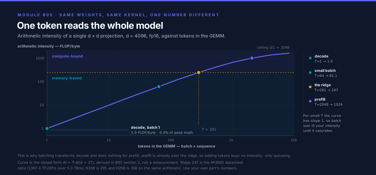
Slope 1 on the left, flat on the right. Everything in this module follows from which side of the bend your workload sits on.
Look at the T = 1 row. You moved 33.6 MB of weights to do 33.6 MFLOP of arithmetic: one FLOP per
byte, on a machine that needs 247 to break even. You are using 0.4% of the available
arithmetic. The matrix cores are idle; the entire cost is the weight read.
And note the middle row: for small T, intensity ≈ T. So the batch size at which decode becomes
compute-bound is roughly the machine's ridge point — a couple of hundred concurrent sequences on
current hardware. That is a remarkably clean result, and it is why serving systems fight so hard for
batch size.
2.5 The prediction that makes this module worth your time¶
If decode is bandwidth-bound and each token requires reading every weight once, then the time per token has a hard floor:
                    model bytes
time per token  ≥  ─────────────
                    HBM bandwidth

                        HBM bandwidth
tokens per second  ≤  ────────────────
                         model bytes
Worked example — Llama-3-8B in fp16 on an MI300X. The model is 8.03 G parameters
(make calc-8b), so 16.06 GB of weights. MI300X HBM3 delivers 5.3 TB/s:
Add the KV cache read for an 8192-token context (1.07 GB) and it falls to 309 tokens/s. On an
H100 SXM (3.35 TB/s) the same model ceilings at 3350 / 16.06 = 209 tokens/s.
Two lines of arithmetic, no code, no GPU — and a real single-stream deployment will land in the low hundreds of tokens/s. Quantize the weights to int8 and the model halves to 8.03 GB, so the ceiling doubles to 660 tokens/s. That is the entire business case for quantization on the decode path, and it follows from one division.
The formula is easy to accept and still design against, because what it does not convey is the repetition — that the same 16 GB is dragged across the bus again for token 2, and token 3, and token 900:
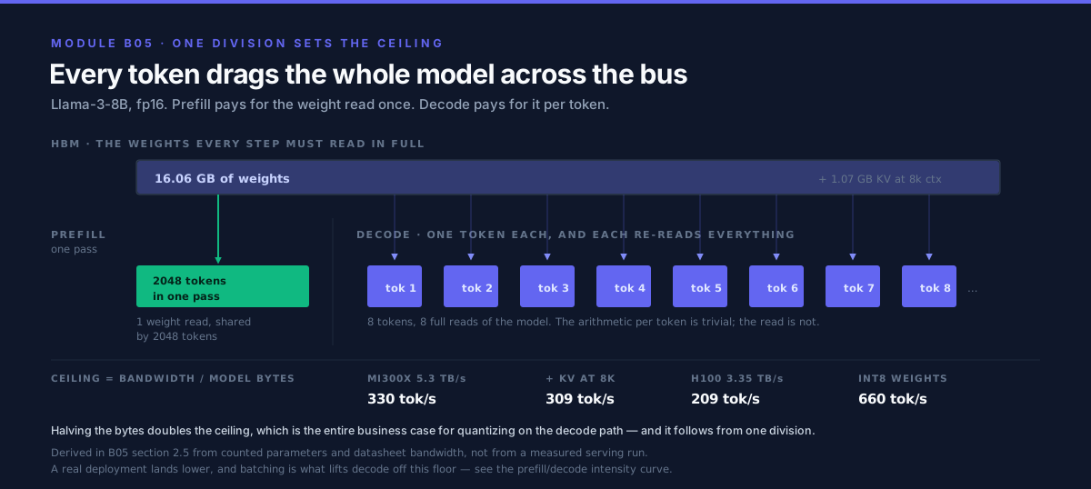
Prefill gets one arrow for the whole prompt. Decode gets one per token, forever.
3. Deep Dive¶
3.1 The two regimes, side by side¶
%%{init: {
  'theme': 'base',
  'themeVariables': {
    'primaryColor': '#F8FAFC',
    'primaryTextColor': '#0F172A',
    'primaryBorderColor': '#0891B2',
    'lineColor': '#64748B',
    'secondaryColor': '#E0F2FE',
    'tertiaryColor': '#EEF2FF',
    'fontFamily': 'Inter, Segoe UI, sans-serif'
  }
}}%%
flowchart TB
  START["Same weights, same model.<br/>How many tokens per forward pass?"]

  START --> PRE["PREFILL / TRAINING<br/>thousands of tokens at once"]
  START --> DEC["DECODE<br/>exactly 1 token per sequence"]

  PRE --> PSHAPE["GEMM shape: (N x d) @ (d x d)<br/>N = 2048+"]
  PSHAPE --> PAI["arithmetic intensity ~1600 FLOP/byte<br/>weight read amortized over N tokens"]
  PAI --> PBOUND["COMPUTE-BOUND<br/>matrix cores are the ceiling"]
  PBOUND --> PFIX["Levers: fused attention, larger tiles,<br/>lower-precision matrix cores, fewer FLOPs"]
  PFIX --> PBATCH["Batching: almost no gain<br/>(already saturating the cores)"]

  DEC --> DSHAPE["GEMM shape: (1 x d) @ (d x d)<br/>a matrix-VECTOR product"]
  DSHAPE --> DAI["arithmetic intensity ~1 FLOP/byte<br/>whole weight read for ONE token"]
  DAI --> DBOUND["MEMORY-BANDWIDTH-BOUND<br/>HBM is the ceiling"]
  DBOUND --> DFIX["Levers: batching, quantization,<br/>smaller KV cache, speculative decoding"]
  DFIX --> DBATCH["Batching: near-LINEAR gain<br/>(one weight read serves B sequences)"]

  classDef trackB fill:#6366F1,stroke:#0F172A,color:#fff
  classDef neutral fill:#F8FAFC,stroke:#0891B2,color:#0F172A
  classDef success fill:#10B981,stroke:#0F172A,color:#fff
  classDef warn fill:#FEF3C7,stroke:#F59E0B,color:#0F172A
  class START neutral
  class PRE,PSHAPE,PAI,DEC,DSHAPE,DAI trackB
  class PBOUND success
  class DBOUND warn
  class PFIX,PBATCH,DFIX,DBATCH neutral
Read the two columns as answers to the same question about the same weights: the only input that changed is the token count per pass, and it moved the bottleneck from the matrix cores to HBM — which inverts the entire optimization list, and inverts whether batching is your best lever or nearly useless.
The opposite bottlenecks below — one arrangement of weights, two ceilings — are derived in full by Pope et al. (2022), which is the source this section follows. The asymmetry in the last row is the practical payoff and the reason B06 exists:
| Prefill / training | Decode | |
|---|---|---|
| Tokens per pass | B × N, thousands |
B, one per sequence |
| Dominant GEMM shape | matrix–matrix | matrix–vector |
| Arithmetic intensity | 10³ FLOP/byte | ~1 FLOP/byte, ≈ B when batched |
| Bottleneck | matrix cores | HBM bandwidth |
| Latency metric | time-to-first-token (TTFT) | inter-token latency (ITL) |
| Effect of doubling batch | ~2× the time, ~same throughput | ~same time, ~2× throughput |
| Effect of halving weight bytes | little | ~2× throughput |
| Effect of 2× faster matrix cores | ~2× | nothing |
The last two rows are the ones that get budget approved or rejected. A vendor slide advertising 2× the FLOPs is advertising a prefill improvement; if your production workload is 10-token prompts and 500-token responses, you are buying almost nothing.
3.2 Inside a layer, with per-stage costs¶
%%{init: {
  'theme': 'base',
  'themeVariables': {
    'primaryColor': '#F8FAFC',
    'primaryTextColor': '#0F172A',
    'primaryBorderColor': '#0891B2',
    'lineColor': '#64748B',
    'secondaryColor': '#E0F2FE',
    'tertiaryColor': '#EEF2FF',
    'fontFamily': 'Inter, Segoe UI, sans-serif'
  }
}}%%
flowchart TB
  IN["x : (B, N, d)"] --> N1["RMSNorm<br/>0 GEMM FLOPs · 2Nd bytes<br/>MEMORY-BOUND"]
  N1 --> QKV["Q, K, V projections<br/>params 2d² + 2·d·d_kv<br/>FLOPs 2N(2d² + 2·d·d_kv)"]
  QKV --> ROPE["RoPE on Q, K<br/>0 GEMM FLOPs · elementwise<br/>MEMORY-BOUND"]
  ROPE --> KV["append K, V to cache<br/>+2·d_kv·dtype bytes per token per layer"]
  KV --> SCORE["QK^T<br/>FLOPs 2N²d · materializes h·N² scores<br/>QUADRATIC in N"]
  SCORE --> SM["softmax<br/>0 GEMM FLOPs · reads+writes h·N²<br/>MEMORY-BOUND, the fusion target"]
  SM --> AV["scores @ V<br/>FLOPs 2N²d"]
  AV --> O["O projection<br/>params d² · FLOPs 2Nd²"]
  O --> R1["residual add<br/>3Nd bytes · MEMORY-BOUND"]
  R1 --> N2["RMSNorm<br/>MEMORY-BOUND"]
  N2 --> FFN1["FFN gate + up<br/>params 2·d·d_ffn · FLOPs 4N·d·d_ffn<br/>the FLOP and byte heavyweight"]
  FFN1 --> ACT["SwiGLU<br/>0 GEMM FLOPs · 3N·d_ffn bytes<br/>MEMORY-BOUND, widest tensor in the layer"]
  ACT --> FFN2["FFN down<br/>params d·d_ffn · FLOPs 2N·d·d_ffn"]
  FFN2 --> R2["residual add<br/>MEMORY-BOUND"]
  R2 --> OUT["out : (B, N, d)"]

  classDef trackB fill:#6366F1,stroke:#0F172A,color:#fff
  classDef warn fill:#FEF3C7,stroke:#F59E0B,color:#0F172A
  classDef neutral fill:#F8FAFC,stroke:#0891B2,color:#0F172A
  class QKV,SCORE,AV,O,FFN1,FFN2 trackB
  class N1,ROPE,SM,R1,N2,ACT,R2 warn
  class IN,OUT,KV neutral
Indigo boxes hold all the parameters and all the FLOPs; amber boxes hold none of the parameters and are pure HBM traffic — and there are seven of them against six GEMMs. The GEMMs decide your FLOP bill, but the amber boxes decide how much of the machine you actually get to use, because each one is a full round trip to HBM for arithmetic that could have been done in registers.
3.3 The elementwise tax, quantified¶
"LayerNorm is cheap" is true in FLOPs and false in time. Add up the HBM traffic of the amber boxes
for one token, one layer of a Llama-3-8B shape (d = 4096, d_ffn = 14336, d_kv = 1024,
bf16 = 2 B/element), counting one read of each input and one write of the output:
| Operation | Elements touched | Bytes |
|---|---|---|
| RMSNorm (pre-attention) | read d, write d |
16,384 |
| RoPE on Q and K | read + write d + d_kv |
20,480 |
| residual add (attention) | read 2d, write d |
24,576 |
| RMSNorm (pre-FFN) | read d, write d |
16,384 |
| SwiGLU activation | read 2·d_ffn, write d_ffn |
86,016 |
| residual add (FFN) | read 2d, write d |
24,576 |
| total | 188,416 B ≈ 188 KB per token per layer |
Compare against the layer's weights: 218.1 M parameters × 2 B = 436 MB. So:
elementwise traffic overtakes the weight read when
    tokens per pass  >  436,207,616 / 188,416  ≈  2,315 tokens
This is the whole argument for fusion, made numerically. In
decode (1–64 tokens per pass) the
elementwise ops are ~0.04% of the traffic and fusing them is a rounding error — spend your effort on
batching instead. In training or prefill with 4k–8k tokens per pass, that same unfused elementwise
traffic exceeds the entire weight read, and fusing norms + activation + residual into their
neighbouring GEMMs
(A07's technique, applied at
model scale) is one of the largest single wins
available. Note also the asymmetry inside the table: SwiGLU alone is 46% of the total, purely
because it operates on the d_ffn-wide tensor rather than the d-wide one.
The lesson generalizes: which optimization is correct depends on the regime, and the same code change can be essential or worthless depending on tokens-per-pass.
3.4 KV cache: the thing that actually limits concurrency¶
During decode you must not recompute K and V for tokens you already processed, so you cache them. Per sequence:
KV bytes = 2 × layers × N × d_kv × dtype_bytes
           │                │
           │                └─ width of ONE of K or V  = kv_heads × d_head
           └─ K and V are two separate tensors
Under MHA, d_kv = d — every query head has its own K/V head. This is expensive, and the fix is
to let several query heads share one K/V head:
| Scheme | KV heads | d_kv |
KV cache size | Quality |
|---|---|---|---|---|
| MHA (Vaswani et al. 2017) | h |
d |
baseline | baseline |
| GQA (Ainslie et al. 2023) | h/g |
d/g |
1/g of MHA |
~MHA with uptraining |
| MQA (Shazeer 2019) | 1 | d_head |
1/h of MHA |
measurable degradation |
Worked example — Llama-2-70B (L = 80, d = 8192, h = 64, kv_heads = 8, d_head = 128;
Touvron et al. 2023, Table 1 and the reference implementation's ModelArgs). So d_kv = 8 × 128 =
1024, an 8× reduction from d = 8192:
GQA :  2 × 80 × 1024 × 2 B  =   327,680 B = 328 KB per token
MHA :  2 × 80 × 8192 × 2 B  = 2,621,440 B = 2.62 MB per token   (8x more)

at N = 4096:
GQA :  328 KB × 4096  =  1.34 GB per sequence
MHA :  2.62 MB × 4096 = 10.74 GB per sequence
Now put it on a GPU. The 70B model in fp16 is 68.98 G params = 137.95 GB, on an MI300X with 192 GB:
free for KV = 192 − 137.95 = 54.05 GB

with GQA :  54.05 / 1.34  =  40 concurrent sequences
with MHA :  54.05 / 10.74 =   5 concurrent sequences
GQA is worth 8× the concurrency, which — because decode throughput scales with batch — is worth close to 8× the serving throughput at the same latency. That is why essentially every model released after 2023 uses GQA or MQA. It is not an accuracy optimization; it is a concurrency optimization that happens to cost little accuracy.
Why the KV cache, not the weights, is the binding constraint. The weights are a fixed
one-time cost: pay 137.95 GB once and serve any number of requests. The KV cache is O(batch × N) —
it grows with both the concurrency you want and the context length you advertise. Double your
advertised context from 4k to 8k and you halve your maximum concurrency, without changing the model
at all. Every serving system's hardest problem is KV-cache management, which is why vLLM's central
contribution was PagedAttention — treating the cache as pageable blocks to eliminate the
fragmentation waste that this simple division ignores
(Kwon et al. 2023).
Run python tools/model_calculator.py --preset llama2-70b --gpu mi300x --batch 32 to reproduce all
of the above, and change --kv-dtype fp8 to see what cache quantization buys.
3.5 Architectural variants, read as performance decisions¶
Every "architecture choice" in a model card is really a decision on this table:
| Variant | Parameters | FLOPs per token | Memory traffic | Why you would do it |
|---|---|---|---|---|
| MHA → GQA | slightly ↓ | ~unchanged | KV cache ÷ g | concurrency; the highest-leverage change on this list |
| MHA → MQA | ↓ | ~unchanged | KV cache ÷ h | maximum concurrency, accept quality loss |
| post-norm → pre-norm | unchanged | unchanged | unchanged | trainability at depth (Xiong et al. 2020) — free |
| LayerNorm → RMSNorm | ↓ (no bias) | ↓ slightly | ↓ slightly | one less pass over the data (Zhang & Sennrich 2019) |
| GELU → SwiGLU | ↑ 50% of FFN | ↑ 50% of FFN | ↑ | better quality per parameter (Shazeer 2020) |
| dense → MoE | ↑↑ 10–100× | ~flat (top-k routing) | ↑↑ | quality at fixed FLOPs — but see below |
Two of these deserve care because they are commonly misread.
SwiGLU is not free. It needs a third matrix (gate, up, down instead of up, down), so the FFN
becomes 3·d·d_ffn rather than 2·d·d_ffn. Implementers compensate by shrinking d_ffn from 4d
to about 8d/3, keeping the parameter count roughly constant. Llama-3-8B
(Grattafiori et al. 2024)
sets d_ffn = 14336 with
d = 4096 — a ratio of 3.5, so the FFN is 3 × 3.5 = 10.5 d² against the textbook 8d². Its
attention block, thanks to GQA, is only 2.5d² instead of 4d². Net: 13.00 d² per layer,
almost exactly the textbook 12d². The two deviations nearly cancel — which is why the crude rule
keeps working on modern models, and why you should know why it works rather than trusting it
blindly.
MoE decouples parameters from FLOPs, and that is a trap as much as a feature. A mixture-of-
experts layer holds E copies of the FFN but routes each token to k of them (Shazeer et al. 2017;
Fedus et al. 2021). Parameters go up ~E/k×; FLOPs per token stay flat. Read that through §2.5:
decode throughput is bandwidth / model_bytes, and MoE multiplied model_bytes while leaving
FLOPs alone. So MoE makes the compute-bound regime cheaper per unit quality and the
bandwidth-bound regime harder. It also introduces load-imbalanced, data-dependent routing —
all-to-all traffic, expert hotspotting, and padding waste — none of which appears in a FLOP count.
MoE is a bet that you will serve at high enough batch to be compute-bound.
3.6 Where the hardware enters¶
The regime boundary is a property of the machine, not the model. It is the roofline ridge point of Williams et al. (2009):
| Accelerator | Dense bf16/fp16 peak | HBM bandwidth | Ridge point | Capacity |
|---|---|---|---|---|
| AMD MI300X | 1307.4 TFLOP/s | 5.3 TB/s | 247 FLOP/byte | 192 GB |
| AMD MI355X | ~2.5 PFLOP/s | 8.0 TB/s | ~313 FLOP/byte | 288 GB |
| NVIDIA H100 SXM | 989.4 TFLOP/s | 3.35 TB/s | 295 FLOP/byte | 80 GB |
| NVIDIA H200 SXM | 989.4 TFLOP/s | 4.8 TB/s | 206 FLOP/byte | 141 GB |
(Vendor-published dense peaks, no sparsity doubling. Confirm against the datasheet for your exact SKU and clock configuration — these move between revisions.)
Three things follow, and they are the architecture-aware part of this module:
- Ridge points are in the low hundreds and have been rising. FLOPs have grown faster than bandwidth for a decade, so the batch size needed to escape the memory-bound regime keeps climbing. Decode gets relatively worse on each generation unless you also batch harder.
- Capacity is the concurrency budget. MI300X's 192 GB versus H100's 80 GB is not a minor spec: from §3.4, a 70B fp16 model leaves 54 GB for KV on an MI300X and does not fit at all on an 80 GB H100 without sharding (B07). Capacity buys batch, and batch is decode throughput.
- Compare H100 and H200. Identical compute, 43% more bandwidth. For prefill that is worth nearly nothing; for decode it is worth ~43% more tokens/s. Same silicon, and which number matters depends entirely on which regime you are serving.
4. Hands-On Labs¶
This module is Python-first: it analyzes and measures transformers rather than writing kernels
(the kernels themselves are
A06 /
A07 /
A09). There is no cuda/,
hip/, or triton/ directory and
nothing to compile. make with no target prints the full list.
make                    # help
make calc               # all presets, analytical (no GPU, no third-party packages)
make profile            # time a decoder layer: prefill vs decode      [needs GPU + torch]
make scaling            # decode throughput vs batch size              [needs GPU + torch]
make run                # calc + both benchmarks
make check              # smoke-test the calculator
tools/ is stdlib-only on purpose — you can size a model on a login node, in a bare container, or
on a laptop during an interview. bench/ needs a GPU and refuses to run on CPU with a message
pointing you back to the calculator, because a CPU timing here would teach the wrong lesson rather
than merely being slow.
Lab 1 — Size a model on paper (tools/model_calculator.py)¶
No GPU required. Everything it prints is a derived estimate from the §2 formulas: an analytical ceiling assuming perfect overlap, zero launch overhead, and 100% of vendor-published bandwidth. Real hardware lands below it.
python tools/model_calculator.py --preset llama3-8b --gpu mi300x
python tools/model_calculator.py --preset llama2-70b --gpu mi300x --batch 32
python tools/model_calculator.py --preset gpt3-175b --gpu h100
# your own architecture:
python tools/model_calculator.py -L 48 -d 6144 --heads 48 --kv-heads 8 \
    --ffn 16384 --glu --vocab 64000 --seq 8192 --gpu mi355x
What to observe. Four things, in this order:
- The
12d²rule survives contact with real models.--preset gpt3-175breports exactly12.00 d²per layer;--preset llama3-8breports13.00 d²despite using both GQA and SwiGLU, because those two deviations nearly cancel (§3.5). - The decode throughput ceiling is a single division and it is close to reality. 8B/fp16 on MI300X: 330 tokens/s.
- The
--dtype int8lever doubles it, because it halves the bytes. Try it — this is the whole quantization argument in one flag. - The
--kv-headslever multiplies concurrency. Run--preset llama2-70band read the "same model with MHA instead" line: 40 sequences versus 5.
Lab 2 — Watch a layer change regime (bench/profile_layer.py)¶
Builds one Llama-style decoder layer (RMSNorm, GQA + RoPE, SwiGLU) from plain torch ops and times each sub-operation twice: once at a prefill shape (2048 new tokens) and once at a decode shape (1 new token, attending over a 2048-token cache). Same weights both times.
python bench/profile_layer.py
python bench/profile_layer.py --hidden 8192 --ffn 28672 --heads 64 --kv-heads 8
python bench/profile_layer.py --prefill-seq 4096 --batch 4 --dtype bfloat16
It warms up before timing (the first call pays lazy init and GEMM heuristic selection — constants
large enough to swamp the decode measurements, which are only tens of microseconds) and times with
torch.cuda.Event, not a host clock, because kernel launches are asynchronous
(A01 §6).
What to observe:
- In the prefill table, the
TFLOP/scolumn is high for the GEMM rows and the FFN rows dominate the time — time is tracking FLOPs, and the FFN holds most of the parameters. - In the decode table, the same GEMM rows show
FLOP/Bcollapsed to ~1 and it is now theGB/scolumn that is large. Same kernels, same weights, opposite bottleneck. - The
us/tokenline at the bottom of each regime differs by two to three orders of magnitude. Decode does ~2048× less work per step but the step is nowhere near 2048× faster. - The reported materialized score matrix size: this is the
O(N²)allocation FlashAttention eliminates. Watch it grow quadratically as you raise--prefill-seq. - The per-category summary: what fraction of the layer is GEMM versus attention versus elementwise. Compare the elementwise share between the two regimes and check it against §3.3's crossover prediction of ~2315 tokens.
The layer is deliberately unfused and does not call a flash-attention kernel — it is the naive baseline that A07 fuses and B06 optimizes. Numbers are per-sub-op; their sum approximates an unfused layer but is not identical to an end-to-end forward pass, which gets some inter-kernel overlap.
Lab 3 — Prove batching amortizes the weight read (bench/batch_scaling.py)¶
The hypothesis from §2.4–2.5, stated as a falsifiable claim: if decode cost is the weight read, then running 32 sequences per step should cost barely more than running 1.
python bench/batch_scaling.py --bandwidth 5300
python bench/batch_scaling.py --layers 16 --batches 1,2,4,8,16,32,64,128,256,512
What to observe — the expected shape, which is the lesson (absolute numbers are yours):
- step latency: nearly flat across the small batch sizes, then bending upward.
- aggregate tokens/s: nearly linear in batch across that flat region.
- weight GB/s: climbs toward a large fraction of peak and holds roughly constant while bandwidth-bound — then falls, which is the signature of having left the regime.
- TFLOP/s: low but rising linearly. The math was never the limit.
- FLOP/B: in fp16 this column equals the batch size exactly (2 FLOPs per weight per token ÷ 2 bytes per weight). Compare it against your machine's ridge point from §3.6 and you can read off where the knee should be before you see it.
The knee — where latency starts growing proportionally with batch — is the crossover to compute-bound, and the calculator predicts roughly where it lands. Finding it, and finding that it sits at a batch size in the hundreds, is the experimental payoff of the whole module.
Attention over the KV cache is deliberately excluded from this benchmark. Its byte count scales with batch (each sequence owns its cache), so including it would mask the effect under test. That interaction is precisely what caps real serving batch sizes, and it is B06's subject.
5. Performance Analysis¶
5.1 Placing both regimes on the roofline¶
%%{init: {
'theme': 'base',
'themeVariables': {
'primaryColor': '#F8FAFC',
'primaryTextColor': '#0F172A',
'primaryBorderColor': '#0891B2',
'lineColor': '#64748B',
'secondaryColor': '#E0F2FE',
'tertiaryColor': '#EEF2FF',
'fontFamily': 'Inter, Segoe UI, sans-serif'
}
}}%%
flowchart LR
subgraph MEM["Memory-bound region — below the ridge point"]
D1["decode, batch 1<br/>~1 FLOP/byte"]
D2["decode, batch 32<br/>~32 FLOP/byte"]
EW["norms, RoPE, SwiGLU, residuals<br/><1 FLOP/byte in every regime"]
end
RIDGE["RIDGE POINT<br/>MI300X ~247 FLOP/byte<br/>H100 ~295 FLOP/byte"]
subgraph COMP["Compute-bound region — above the ridge point"]
D3["decode, batch 512<br/>~512 FLOP/byte"]
P1["prefill N=2048<br/>~1024 FLOP/byte"]
TR["training, 8k tokens/microbatch<br/>~1600 FLOP/byte"]
end
D1 --> D2 --> RIDGE --> D3 --> P1 --> TR
EW -.->|"never crosses:<br/>fusion is the only fix"| RIDGE
classDef trackB fill:#6366F1,stroke:#0F172A,color:#fff
classDef warn fill:#FEF3C7,stroke:#F59E0B,color:#0F172A
classDef success fill:#10B981,stroke:#0F172A,color:#fff
classDef neutral fill:#F8FAFC,stroke:#0891B2,color:#0F172A
class D1,D2,EW warn
class RIDGE neutral
class D3,P1,TR success
class COMP,MEM trackBOne model occupies the entire horizontal span of the roofline depending only on tokens-per-pass — so "optimize the transformer" is meaningless until you say where on this line you are sitting. Note that the elementwise ops sit permanently on the left and cannot be batched across the ridge: no batch size raises their intensity, because they read and write proportionally to their own output. Fusion is the only lever that moves them, which is why it is A07's whole subject.
5.2 Analytical results (derived — not measured)¶
Produced by tools/model_calculator.py, which evaluates §2's formulas. These are ceilings, not
benchmarks: perfect overlap, no launch overhead, full published bandwidth. Reproduce with
make calc.
Llama-3-8B shape (32 layers, d = 4096, 32 heads, 8 KV heads, d_ffn = 14336, vocab 128256):
| Quantity | Derived value | Where it comes from |
|---|---|---|
| Parameters per layer | 218.1 M (13.00 d²) |
§2.1, GQA + SwiGLU |
| Total parameters | 8.03 G | matches the published "8B" |
| Weights, fp16 | 16.06 GB | params × 2 B |
| Forward FLOPs per token | 13.96 GFLOP | 2 × non-embedding params |
| Training FLOPs per token | 41.88 GFLOP | 6 × non-embedding params |
| KV cache per token | 131.1 KB | 2 × 32 × 1024 × 2 B |
| KV cache at N=8192 | 1.07 GB per sequence | above × 8192 |
| Attention/FFN FLOP crossover | N ≈ 26,624 tokens | p_layer / 2d |
| Decode ceiling, MI300X | 330 tokens/s | 5300 / 16.06 |
| Decode ceiling, H100 | 209 tokens/s | 3350 / 16.06 |
| Decode ceiling, MI300X, int8 | 660 tokens/s | weights halve |
| Batch for compute-bound decode | ~280 sequences | intensity ≈ ridge point |
Llama-2-70B shape on a single 192 GB MI300X:
| Quantity | Derived value |
|---|---|
| Total parameters | 68.98 G |
| Weights, fp16 | 137.95 GB |
| HBM left for KV | 54.05 GB |
| KV per sequence at N=4096, GQA | 1.34 GB → 40 concurrent |
| KV per sequence at N=4096, MHA | 10.74 GB → 5 concurrent |
| Decode ceiling, batch 1 | 38 tokens/s |
| Decode ceiling, batch 32 | 938 tokens/s aggregate, 29 per sequence |
Read the last two rows together: 32× the batch bought 24× the aggregate throughput while per-user speed only fell from 38 to 29 tokens/s. That trade — a small latency concession for a large throughput gain — is the single most important economic fact in LLM serving, and it exists only because decode is bandwidth-bound.
5.3 Measured results — run them yourself¶
There is no measured table in this README on purpose. Timings depend on GPU, ROCm/CUDA version,
torch version, clocks, and thermal state, and a copied-in number would be a fabrication rather than
evidence. Run make profile and make scaling on your hardware and expect these shapes:
| Measurement | Expected shape | What confirms the theory |
|---|---|---|
profile_layer, prefill |
GEMM rows dominate; high TFLOP/s | time tracks FLOPs |
profile_layer, decode |
same rows, FLOP/B ≈ 1, high GB/s |
time tracks bytes |
profile_layer, µs/token |
100–1000× worse in decode | the weight read, unamortized |
batch_scaling, latency |
flat, then a knee | fixed weight read, then compute |
batch_scaling, throughput |
near-linear before the knee | batching amortizes the read |
batch_scaling, weight GB/s |
rises to a plateau, then falls | HBM is the limiter, until it isn't |
batch_scaling, knee location |
batch in the hundreds | matches the ridge point |
If your measured single-stream tokens/s is far below the calculator's ceiling, that gap is the finding — and it is what B03's profilers are for. The usual causes, in order of frequency: kernel launch overhead dominating tiny decode kernels (fix: CUDA/HIP graphs), unfused elementwise ops, a Python-side bottleneck between steps, and memory layouts that fail to coalesce (A02).
6. Challenges, Drawbacks & Tradeoffs¶
%%{init: {
  'theme': 'base',
  'themeVariables': {
    'primaryColor': '#F8FAFC',
    'primaryTextColor': '#0F172A',
    'primaryBorderColor': '#0891B2',
    'lineColor': '#64748B',
    'fontFamily': 'Inter, Segoe UI, sans-serif'
  }
}}%%
flowchart TD
  Q{"Transformer too slow.<br/>Which regime?"}
  Q -->|"long prompts, training,<br/>high TFLOP/s in profiler"| CB["COMPUTE-BOUND"]
  Q -->|"1 token at a time,<br/>low TFLOP/s, high GB/s"| MB["BANDWIDTH-BOUND"]
  Q -->|"OOM before it is slow"| CAP["CAPACITY-BOUND"]

  CB --> CB1["Fuse attention (FlashAttention)"]
  CB --> CB2["Lower-precision matrix cores (fp8)"]
  CB --> CB3["Fuse norms + activations into GEMMs"]
  CB --> CB4["Do NOT bother batching harder"]

  MB --> MB1["Batch aggressively (continuous batching)"]
  MB --> MB2["Quantize WEIGHTS (int8/int4)"]
  MB --> MB3["Shrink KV cache: GQA/MQA, fp8 cache"]
  MB --> MB4["Speculative decoding: more tokens per weight read"]
  MB --> MB5["Do NOT buy more FLOPs"]

  CAP --> CAP1["KV cache is usually the culprit, not weights"]
  CAP --> CAP2["PagedAttention to kill fragmentation"]
  CAP --> CAP3["Shard across GPUs (B07)"]

  classDef trackB fill:#6366F1,stroke:#0F172A,color:#fff
  classDef warn fill:#FEF3C7,stroke:#F59E0B,color:#0F172A
  classDef success fill:#10B981,stroke:#0F172A,color:#fff
  class Q warn
  class CB,MB,CAP trackB
  class CB1,CB2,CB3,CB4,MB1,MB2,MB3,MB4,MB5,CAP1,CAP2,CAP3 success
Pitfall 1 — Optimizing the wrong regime¶
The most expensive mistake in this module's subject area. Teams buy FLOPs for a decode-bound service, or hand-fuse elementwise kernels for a workload where they are 0.04% of traffic (§3.3). Always establish the regime first, with two numbers: tokens per forward pass, and achieved FLOP/byte. Everything else follows.
Pitfall 2 — Quoting one tokens/second number¶
"This model does 300 tokens/s" is meaningless without batch size, context length, and whether it counts prefill. Per-sequence and aggregate throughput differ by the batch size; a benchmark that generates 10 tokens after a 4000-token prompt is measuring prefill and calling it decode. Always report batch, prompt length, generated length, and whether TTFT is included.
Pitfall 3 — Believing 2 × params too literally¶
The rule ignores three things that eventually bite: the 4N²d attention term (§2.3, matters beyond
N ≈ (2+m)d), the 2 × vocab × d lm_head (significant for small models with large vocabularies —
Llama-3-8B's embeddings are 13% of its parameters), and everything memory-bound (§3.3). It is a
first estimate. Its value is that it is right within ~10% for the FLOP-dominant term and takes 20
seconds.
Pitfall 4 — Sizing the KV cache without the runtime's overhead¶
2 × L × N × d_kv × bytes is the floor. A real serving stack adds block-granularity rounding,
fragmentation, a fixed reserve, CUDA-graph pools, and activation scratch. Provisioning at exactly
your computed maximum concurrency will OOM in production. Compute the number, then leave headroom —
and read §3.4's PagedAttention note for why the waste is not a constant factor.
Pitfall 5 — Ignoring launch overhead in decode¶
A decode step for a 32-layer model is hundreds of tiny kernels, each doing a few tens of
microseconds of work. Launch overhead of a few microseconds each is then a significant fraction of
the step. This is why CUDA/HIP graphs and torch.compile matter disproportionately for decode, and
why a naive PyTorch decode loop can land far below the bandwidth ceiling while the GPU sits idle
between kernels. If your measured tokens/s is well under the ceiling and the profiler shows gaps,
this is your bug — not bandwidth.
Pitfall 6 — Treating MoE parameters as free¶
Covered in §3.5: MoE holds FLOPs flat but multiplies bytes, and decode pays for bytes. An MoE model can be slower per token in single-stream decode than a dense model with a tenth the parameters, while being far cheaper at high batch. Know which regime you are buying for.
Tradeoffs worth holding in mind¶
- Batch size: throughput ↑, per-user latency ↑, KV memory ↑ linearly. There is an optimum, it is workload-specific, and it is the central tuning decision in B06.
- Context length: capability ↑, KV cache ↑ linearly, attention FLOPs ↑ quadratically, maximum concurrency ↓. Advertising a 128k context is a serving cost decision disguised as a feature.
- Quantization: bytes ↓ so decode throughput ↑ proportionally; accuracy ↓ by an amount that depends heavily on method and on what you quantized (weights, activations, or the KV cache are three different decisions). B04 is the authority here.
- GQA group size: KV ÷ g and concurrency × g against a quality cost that grows with
g— MQA (g = h) is the aggressive end and is measurably worse than GQA at moderateg.
7. Real-World Use Cases¶
- Capacity planning. "How many GPUs to serve 10,000 concurrent users at 30 tokens/s?" is answered with §2.5 and §3.4 and nothing else: bandwidth ÷ model bytes gives per-GPU token rate, capacity minus weights over KV-per-sequence gives per-GPU concurrency, and the more binding of the two sets your fleet size. This calculation, done in a meeting, routinely changes hardware decisions worth millions.
- Inference serving stacks. vLLM, SGLang, and TensorRT-LLM are, architecturally, machines for exploiting §3.1's asymmetry: continuous batching to keep the decode batch full, PagedAttention to fit more sequences in the KV budget, and chunked prefill / prefill–decode disaggregation so that compute-bound prefill does not stall bandwidth-bound decode. B06 builds this.
- Why FlashAttention exists. §2.3's
O(N²)materialized score matrix — 4.3 GB for a single layer atN = 8192— is not merely slow, it is unallocatable at long context. FlashAttention tiles the computation so the score matrix never leaves on-chip memory (Dao et al. 2022). A07 builds the online-softmax core of it. - Model design. GQA, MQA, sliding-window and other sparse attention patterns, and MLA are all §3.4's arithmetic driving an architecture decision. Ainslie et al. (2023) motivate GQA explicitly in inference-cost terms, not quality terms.
- Speculative decoding. Reads directly off §2.4: if a decode step is bandwidth-bound, verifying
kdraft tokens costs almost the same as generating 1, because the weight read is the cost and it is shared. The speedup comes from raising tokens-per-weight-read, exactly like batching. - The quantization business case. §2.5's division is why int8/fp8/int4 weight quantization became universal for serving: it is the only lever that improves decode throughput without increasing latency or memory pressure, unlike batching, which trades against both.
Where to go next. B06 turns this module's decode arithmetic into a serving system — continuous batching, PagedAttention, and speculative decoding all exist to buy back the tokens-per-weight-read that §2.4 says you are missing. B04 supplies the other half of §2.5's halve-the-bytes lever: which formats survive the accuracy budget, and where fp8 differs between vendors. B07 picks up where one GPU stops — the 70B model that does not fit in §3.6's capacity column, and the interconnect traffic that sharding adds.
8. Cited References¶
Sources shared with other modules are cited by anchor into the master bibliography, where the URL and its retrieval date live; sources only this module uses carry their URL here.
Architecture
- Attention Is All You Need (Vaswani et al., 2017) — the original architecture, and the source of the tensor shapes §2.1 counts parameters from; also the MHA baseline the KV-cache table in §3.4 measures GQA and MQA against.
- Shazeer (2019). Fast Transformer Decoding: One Write-Head is All You Need — MQA, and the first clear statement that the KV cache is the decode bottleneck. https://arxiv.org/abs/1911.02150
- Multi-query and grouped-query attention (Ainslie et al., 2023)
— GQA and the
1/gKV reduction §3.4 turns into a concurrency multiplier, and the argument in §7 that GQA is an inference-cost decision rather than a quality one. - Shazeer (2020). GLU Variants Improve Transformer — SwiGLU and the third FFN matrix (§3.5). https://arxiv.org/abs/2002.05202
- Zhang & Sennrich (2019). Root Mean Square Layer Normalization — RMSNorm. https://arxiv.org/abs/1910.07467
- Su et al. (2021). RoFormer: Enhanced Transformer with Rotary Position Embedding — RoPE, one of §3.3's memory-bound elementwise ops. https://arxiv.org/abs/2104.09864
- Xiong et al. (2020). On Layer Normalization in the Transformer Architecture — pre-norm vs post-norm. https://arxiv.org/abs/2002.04745
- Shazeer et al. (2017). Outrageously Large Neural Networks: The Sparsely-Gated Mixture-of-Experts Layer — MoE. https://arxiv.org/abs/1701.06538
- Fedus, Zoph & Shazeer (2021). Switch Transformers — MoE at scale, top-1 routing. https://arxiv.org/abs/2101.03961
Performance and serving
- Efficiently Scaling Transformer Inference (Pope et al., 2022) — the canonical treatment of the prefill/decode split, the arithmetic intensity of decode, and batching; the direct source for §3.1's two-regime table. Read it if you read only one paper here.
- FlashAttention (Dao et al., 2022)
— why §2.3's
O(N²)materialized score matrix, not attention's FLOP count, is the real problem, and the IO-aware tiling that removes it. - PagedAttention and vLLM (Kwon et al., 2023) — KV-cache fragmentation as the limit on concurrency, and why §3.4's simple division understates the waste in a real serving stack.
- Roofline (Williams et al., 2009) — the ridge point that decides which regime you are in, used throughout §2.4, §3.6 and §5.1.
Scaling laws — the 6N heuristic
- Scaling laws for neural language models (Kaplan et al., 2020)
— source of the
C ≈ 6NDestimate §2.2 derives from the forward/backward FLOP split (see its Table 1 / Appendix compute accounting). - Training compute-optimal large language models (Hoffmann et al., 2022)
— Chinchilla; uses the same
6NDaccounting to derive the compute-optimal token budget, which is what makes §2.2's heuristic worth memorizing rather than looking up.
Model configurations quoted in this module
Every config below was checked against its primary source before being used; the calculator prints the citation alongside each preset.
- Brown et al. (2020). Language Models are Few-Shot Learners — GPT-3 175B: 96 layers,
d = 12288, 96 heads, MHA (Table 2.1). Used in §2.1's12d²validation. https://arxiv.org/abs/2005.14165 - Touvron et al. (2023). Llama 2: Open Foundation and Fine-Tuned Chat Models — Llama-2-70B: 80
layers,
d = 8192, 64 heads, 8 KV heads (GQA),d_ffn = 28672, vocab 32000, 4k context (Table 1 plus the reference implementation'sModelArgs). Used in §3.4. https://arxiv.org/abs/2307.09288 - The Llama 3 herd of models (Grattafiori et al., 2024)
— Llama-3-8B: 32 layers,
d = 4096, 32 heads, 8 KV heads (GQA),d_ffn = 14336, vocab 128256, untied embeddings, 8k context. Config values cross-checked against the published Llama 3 model card andconfig.json. This is the shape every worked example in §2.5, §3.3, §3.5 and §5.2 uses.
Hardware specifications
- AMD Instinct MI300X / MI355X product pages — HBM capacity, bandwidth, and dense matrix-core peaks used in §3.6. https://www.amd.com/en/products/accelerators/instinct.html (retrieved 8 Aug 2026)
- NVIDIA H100 / H200 datasheets — same figures for the Hopper column. https://www.nvidia.com/en-us/data-center/h100/ (retrieved 8 Aug 2026)
9. Self-Assessment & Interview Drills¶
Conceptual¶
- A decoder layer has
d = 8192and an FFN multiplierm = 4, using MHA. How many parameters is the layer, and how many forward FLOPs per token? - You are told a model has 13 B parameters and you must estimate the FLOPs to train it on 1 T tokens. Do it in your head, and say what you are ignoring.
- The classic. Estimate the single-stream generation speed of a 70 B-parameter model in fp16 on one MI300X (5.3 TB/s HBM). Then say what changes if you serve it in int8, and what changes if you batch 32 requests.
- Attention is
O(N²)and the FFN isO(N). Ford = 4096, m = 4, at what sequence length does attention overtake the FFN in FLOPs? Is a 4096-token context above or below that? - Your team doubles the matrix-core throughput of its accelerator with no change to HBM bandwidth. Which of your workloads gets faster: training, prefill, batch-1 decode, batch-512 decode?
- A model uses GQA with 8 KV heads instead of 64. What exactly does that buy, and what is the mechanism by which it improves serving throughput (not just memory)?
- Why does batching help decode enormously but prefill barely at all? Answer in terms of arithmetic intensity.
- LayerNorm has almost no FLOPs. Give a concrete scenario where LayerNorm and friends nevertheless account for more HBM traffic than reading the entire weight matrix, and one where they are negligible.
- An MoE model has 8× the parameters of a dense model but the same FLOPs per token. Which is faster at batch 1, and which at batch 1024? Why?
- Explain to a non-engineer, in three sentences, why generating text is slow but reading a long document is fast, on the same hardware.
Answers
(4 + 2m)d² = 12d² = 12 × 8192² = 12 × 67.1 M = 805 M parameters. FLOPs per token= 2 × params = 1.61 GFLOP. (Attention's4N²dterm is separate and depends onN.)C ≈ 6ND = 6 × 13e9 × 1e12 = 7.8e22 FLOPs. Ignoring: the attentionN²term, the lm_head, activation recomputation (which adds roughly another forward pass, so ~8NDwith full checkpointing), optimizer overhead, and any gap between achieved and peak FLOP/s. As a wall-clock estimate you also need effective (not peak) throughput — typically 30–50% of peak.- 70 B params × 2 B = 140 GB of weights. Decode reads them all per token, so
5300 GB/s ÷ 140 GB ≈ 38 tokens/s. int8: 70 GB, so ~76 tokens/s — bytes halved, ceiling doubled. Batch 32: the weight read is shared, so aggregate throughput goes to roughly32 × 38 ≈ 1200 tokens/s, but per-user speed stays near 38 (falling somewhat as the KV cache reads and activation traffic add up — the calculator gives ~29 for a 4k context). Also note 140 GB of weights leaves only ~52 GB for KV on a 192 GB card, which is what actually caps the batch. N = (2 + m)d = 6d = 24,576tokens. A 4096-token context is far below it — at 4k, attention is a modest fraction of the FLOPs. This is why "attention is the expensive part" is usually wrong about FLOPs and usually right about memory.- Training and prefill get faster (they are compute-bound). Batch-1 decode gets exactly no faster — it is bandwidth-bound and the matrix cores were already idle. Batch-512 decode is likely past the ridge point, so it improves too. This is why the answer to "is the new GPU better" is "for which regime?"
- It cuts the KV cache by 8× (
d_kvgoes fromdtod/8). Mechanism: the KV cache, not the weights, is what consumes the HBM left over after loading the model, so an 8× smaller cache means ~8× more concurrent sequences fit — and since decode throughput scales with batch, ~8× the aggregate throughput at the same latency. It is a concurrency optimization, not a bandwidth one. - Decode's arithmetic intensity is ≈ 1 FLOP/byte, hundreds of times below the ridge point, and batching multiplies it by roughly the batch size — so batching moves you toward the compute ceiling and each doubling roughly doubles throughput. Prefill's intensity is already ~10³ FLOP/byte, well above the ridge point, so the matrix cores are already the limit and batching adds proportional work for proportional time: more throughput per step, but no better throughput per second.
- Significant: training or prefill with thousands of tokens per pass. From §3.3, the elementwise HBM traffic is ~188 KB per token per layer against a 436 MB weight read, so beyond ~2,300 tokens per pass the elementwise ops move more bytes than the weights. Negligible: batch-1 decode, where 188 KB against 436 MB is ~0.04%. Same code, same layer — the regime decides.
- Batch 1: the dense model wins, and by a lot. Decode is bandwidth-bound and the MoE has 8× the bytes to read (routing means you touch fewer experts per token, but the weights still occupy HBM and the achieved read pattern is far less efficient than a dense sweep). Batch 1024: the MoE wins — compute-bound at that batch, and it delivers more quality per FLOP. MoE is a bet on serving at high batch.
- Reading a document lets the machine work on thousands of words simultaneously, so it spends its time doing arithmetic — which is what it is good at. Writing must produce one word before it can start the next, and each single word requires the machine to page through its entire memory of what it has learned. So writing is limited by how fast it can read its own memory, not by how fast it can think.
Coding & Algorithms drills¶
Do these in exercises/; reference answers with full working in
solutions/. All three are paper drills — the skill being tested is producing correct
arithmetic under time pressure on a whiteboard, which is exactly the interview format. Use
tools/model_calculator.py only to check yourself afterwards.
- Size a model (
01_size_a_model.md) — from a config, derive parameters, weight memory in fp16 and int8, prefill versus decode FLOPs, and the predicted decode tokens/s on a given GPU. - KV-cache budget (
02_kv_cache_budget.md) — given HBM capacity, weights, and a target context length, compute maximum concurrency under MHA versus GQA, then state what you would change to double it. - Regime diagnosis (
03_regime_diagnosis.md) — five profiler-style observations. For each: prefill/compute-bound or decode/bandwidth-bound, and the right optimization. Includes cases where the obvious answer is wrong.
Stretch¶
- Extend
tools/model_calculator.pyto model MoE: add--expertsand--top-k, keep FLOPs at the top-kcount while parameters and bytes scale withE, and confirm §3.5's claim that decode throughput degrades while prefill throughput per parameter improves. - Add a tensor-parallel flag: divide weight bytes and FLOPs by the TP degree, but add the
all-reduce traffic (two per layer,
2 × B × N × d × byteseach). Find the TP degree where interconnect traffic starts dominating — then check your answer against B07. - Use
bench/batch_scaling.pyto find your machine's empirical knee, and compare it to the ridge point you compute from the datasheet. If they disagree by more than ~2×, profile (B03) and explain the gap — the usual culprit is launch overhead, not bandwidth. - Reproduce §3.3's crossover experimentally: sweep
--prefill-seqinbench/profile_layer.pyand find the token count at which the elementwise category's share of time stops falling.